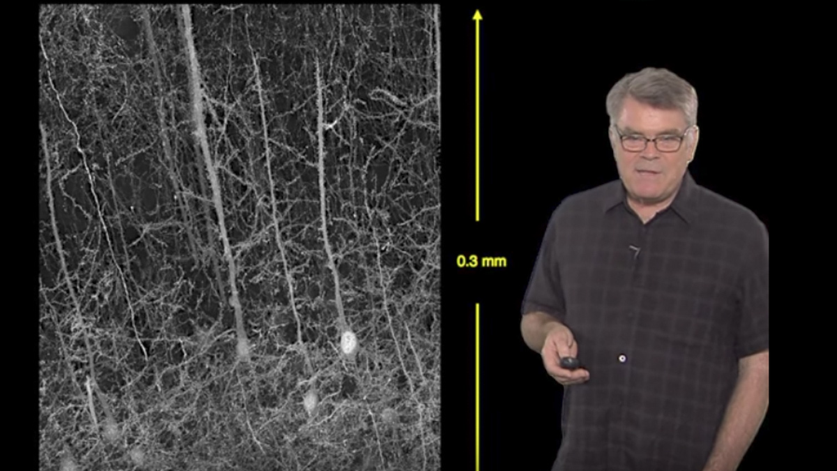
• Skip to primary navigation
  • Skip to main content
  • Skip to primary sidebar
  • Skip to footer

iBiology

Bringing the World's Best Biology to You

  • Start Here
    • Explore iBiology
    • All Playlists
    • All Speakers
    • All Talks
    • What’s new at iBiology?
  • Research Talks
    • Talks by Topic
      • Biochemistry
      • Bioengineering
      • Biophysics
      • Cell Biology
      • Development and Stem Cells
      • Ecology
      • Evolution
      • Genetics and Gene Regulation
      • Human Disease
      • Immunology
      • Microbiology
      • Neuroscience
      • Plant Biology
      • Techniques
      • Archive
    • Talks by Series
      • Bench to Bedside
      • Famous Discoveries
      • Great Unanswered Questions
      • Microscopy Series
      • Share Your Research Series
  • Stories
    • Background to Breakthrough
    • Interviews and Profiles
    • Science and Society
  • Courses
  • Careers
    • Professional Development Talks
    • Professional Development Courses
    • Career Exploration
    • NRMN Resources
    • Biomedical Workforce
  • Educators
  • About
    • Mission
    • Commitment to Inclusion
    • iBiology Team
    • Board of Directors
    • iBiology Funders and Partnerships
    • Contact Us
  • Donate
Home » Courses » Microscopy Series » Specialized Microscopy

Miniature Microscopes for Deep Tissue Imaging

  • Duration: 38:44
  • Downloads
    • Hi-Res
    • Low-Res
  • Subtitles
    • English
  • Transcript

00:00:11.15 Hi, I'm Mark Schnitzer from the Stanford University Department of
00:00:14.18 Applied Physics and the Department of Biology.
00:00:16.15 And the Howard Hughes Medical Institute.
00:00:18.26 And I'm going to be describing today some microscopy techniques
00:00:22.07 that our lab has developed for imaging cells and their attributes
00:00:25.09 deep within the tissues of live animal subjects. And also in
00:00:29.17 animal subjects that are free to behave about the laboratory.
00:00:32.01 My lab focuses on issues pertaining to neuroscience.
00:00:34.29 Particularly at the circuit level, and I think we would all tend to
00:00:38.10 agree that brain circuits remain deeply mysterious.
00:00:41.22 Nonetheless, some of the brain's most fascinating properties
00:00:45.01 arise from the circuit attributes. The numbers involved in trying to
00:00:49.24 dissect neurocircuit function are daunting indeed. In the human brain
00:00:53.01 there are approximately 100 billion neurons and over 100 trillion
00:00:56.15 synapses. So these numbers post some severe challenges.
00:00:59.08 Nonetheless, we have to develop approaches towards understanding
00:01:02.14 how do we learn, and as a result, talk a little bit in this lecture,
00:01:05.23 how do we control our body movements.
00:01:08.07 One of the things that has been badly missing in neuroscience
00:01:10.27 is information about what I'll call the brain's cellular orchestra.
00:01:14.19 We would like to know what are the large-scale, dynamic patterns
00:01:18.00 of activity across a large population of individual cells, and how these
00:01:22.10 dynamic patterns influence animal behavior. Towards attaining
00:01:27.08 such information, we need to have imaging techniques or microscopy
00:01:31.20 techniques that are capable of inspecting cells and watching their dynamics
00:01:35.11 in awake behaving animals. However, traditionally a challenge
00:01:39.02 has been that the classical, or conventional, light microscope has not
00:01:42.25 been well-suited to studies in awake behaving animals.
00:01:45.13 So therefore, traditionally at least, if you want to be able to inspect
00:01:50.20 cells in the live mammalian brain, you might do this in anesthetized
00:01:55.03 animal subject. And this is a Far Side cartoon which provides the physicist's
00:01:59.11 view of this. The caption reads, "What about that! His brain still uses
00:02:02.11 the old vacuum tubes." But ideally, we'd like to be able to inspect
00:02:06.02 cells, not just in anesthetized subjects, but in animal subjects that are
00:02:09.18 free to move about the laboratory and do interesting things. And to
00:02:12.23 look at cells not just in the superficial brain areas that conventional
00:02:16.16 light microscopes can do well, but also in deeper brain areas that lie
00:02:20.23 beyond the penetration depth of the conventional microscopy
00:02:23.20 techniques. So the two main challenges here are the ability to
00:02:27.04 inspect cells that lie deep in tissue, and the ability to observe cells
00:02:30.10 and their dynamics not just in live subjects, but in animal subjects that are
00:02:33.17 free to move about the laboratory. And I will discuss these two
00:02:36.22 technical dilemmas in turn. The first technical challenge here is
00:02:40.21 how do we perform cellular level imaging with micron-scale resolution
00:02:44.14 in deep tissues and in vivo? And when I say in vivo here, I mean
00:02:48.14 generally in the live mammalian brain. And this slide illustrates some of the
00:02:53.21 optical challenges involved. Light scattering is actually the chief
00:02:57.17 impediment, not light absorption. These outer colored bands
00:03:02.13 indicate the range of tissue that are accessible to conventional light
00:03:05.28 microscopy techniques. So for example, if you wish to inspect
00:03:09.13 cells with a conventional confocal fluorescence microscope,
00:03:12.22 you can observe cells in approximately the outer few hundred microns of
00:03:16.18 tissue, as illustrated here with this orange band in this sagittal view
00:03:20.26 of the rat brain. The two-photon fluorescence microscope can do much
00:03:24.18 better, as indicated here by this green band. The two-photon microscope
00:03:29.07 can penetrate about 500-700 microns, maybe a little bit more
00:03:32.22 on a very good day, deep into brain tissue. But I think you can see that the
00:03:36.07 vast majority of the mammalian brain actually lies out of reach of
00:03:39.25 these conventional microscopy techniques. And so the question thus
00:03:43.10 is, how do we inspect cells in deeper lying areas that pertain to many
00:03:47.24 brain diseases, how do we look at cells in deep areas such as the
00:03:50.18 hippocampus, the basal ganglia, and many other areas of interest.
00:03:53.20 Well, over the last few years, my group has developed techniques
00:03:57.02 that we call, "microendoscopy." And the microendoscopy method
00:04:00.23 had made use of fluorescence contrast modalities, as well as some
00:04:03.28 other contrast modalities such as second harmonic generations.
00:04:06.14 And I'll discuss these as we proceed.
00:04:08.21 This slide here illustrates some of the micro-optical probes
00:04:12.03 that our lab has explored for imaging cells that lie deep in the
00:04:15.10 brain. This probe here, is a thousand microns in diameter.
00:04:19.27 This one is 350 microns in diameter, and it's poised to go into Abraham
00:04:25.04 Lincoln's brain. At the tip of each probe, you can see a tiny little
00:04:30.02 micro-optical objective that provides the micron-scale resolution
00:04:35.05 that we need to see cells in deep-lying locations. And in each
00:04:38.26 case, this micro-optical objective is followed by a longer
00:04:42.06 but weaker relay lens, whose main purpose is to give us
00:04:45.18 the reach we need to penetrate deep within the tissue.
00:04:48.20 Before I go into the details about how these micro-optical
00:04:52.05 probes work. I'm going to show you an example set of videos
00:04:55.21 that illustrate what you can observe in the living brain looking through
00:05:00.00 these optical needles, these micro-optical probes. In the first video
00:05:04.05 you're going to see a low magnification view of microcirculation
00:05:08.07 in the vascular network in a deep brain area, hippocampal CA1.
00:05:12.09 In a live rodent. We've performed an intravascular injection of
00:05:16.27 a fluorescent dye, fluorescein, the dye will label the blood plasma brightly,
00:05:21.19 whereas the red blood cells will appear dark in relief. And you're
00:05:25.03 going to be able to see them flowing through the individual capillaries.
00:05:28.14 In the first video, we've inserted a low-magnification optical needle
00:05:33.22 into the tissue, but already at this low-magnification, you can already
00:05:37.15 make out the structure of the microvasculature, the directions
00:05:40.14 of flow, relative speeds, and so forth. We can now hot swap the
00:05:46.06 optical probes, pulling this low-magnification probe out of the brain
00:05:49.20 and replacing it with a probe of higher magnification.
00:05:53.00 Here in this slide, now you can see the individual red blood cells
00:05:57.09 passing single file through the capillaries in this live brain.
00:06:01.23 We can now replace the micro-optical probe again, inserting a
00:06:06.08 higher magnification optical needle, and here at the very highest
00:06:10.26 magnification, you can clearly see the individual red blood
00:06:14.22 cells passing through the capillary. And if I stop the video, to give you
00:06:19.12 a closer look at one of these erythrocytes, you can see
00:06:22.04 that the individual cells, which we know to be about 8-microns in
00:06:26.09 extant, actually appear to be broader than the capillary itself.
00:06:30.12 And that gives you a sense of the kind of micron scale details that
00:06:34.09 we can see in real time looking through one of these micro-optical needles.
00:06:38.12 Building on these basic capabilities for micro-optical imaging,
00:06:42.00 we have extended our imaging capacities in several different
00:06:46.08 directions. First, we've come up with a chronic mouse preparation
00:06:49.28 that allows us to perform time-lapse or longitudinal imaging at the cellular
00:06:55.08 scale. Returning again and again to the same site of the brain,
00:06:59.04 the same cells, the same neuronal dendrites, and in some cases, even
00:07:02.20 the same synapses. In most mice, we're able to do this for a period
00:07:06.01 of two months. Occasionally, we've been able to follow cells in
00:07:10.09 an individual mouse for periods of up to a year.
00:07:12.22 Secondly, we have been able to combine the micro-optical lenses that
00:07:17.12 I've been discussing with other small elements, such as micro-fabricated laser
00:07:21.28 scanning mirrors, that have allowed us to put together a small mouse-sized
00:07:25.23 two-photon microscope with a mass of approximately 2.5 grams.
00:07:30.05 And complementary to this small device is another instrument, a
00:07:34.00 high-speed 1.1 gram epifluorescence microscope that I will describe
00:07:38.02 towards the latter half of the lecture. Let's start off by examining
00:07:43.04 the means by which these micro-optical needles are able to provide
00:07:46.25 micron scale views of cells deep within living tissue. And our early
00:07:51.27 work in this regard was done by Juergen Jung in the lab.
00:07:54.23 Together, we developed two different contrast modalities for fluorescence
00:07:59.01 microendoscopy deep in living tissue. These two modalities
00:08:04.11 are the epifluorescence version of microendoscopy, and the
00:08:08.25 second one is the laser scanning two-photon variety of microendoscopy.
00:08:13.20 And they have complementary sets of strengths and limitations.
00:08:17.07 The epifluorescence form functions very similarly to the epifluorescence
00:08:23.11 microscope that many of you may already be familiar with.
00:08:27.06 Except that we have this long skinny probe for delivering illumination
00:08:32.10 deep into the brain, and for receiving images of the cells.
00:08:38.09 This epifluorescence version of microendoscopy uses a standard
00:08:43.10 dichroic filter set, standard sources of illumination, such as a mercury
00:08:46.23 arc lamp. And its virtues, first of all, its simplicity and the fact that we can
00:08:51.16 acquire full-frame images at relatively fast frame rates.
00:08:55.15 So, for example, my laboratory regularly uses this modality
00:08:59.12 at frame rates of approximately 100 Hertz, sometimes extending to
00:09:03.08 over a kiloHertz. However, a disadvantage of fluorescence microendoscopy
00:09:08.22 is that like conventional epifluorescence microscopy, this modality
00:09:13.07 is not terribly robust to light-scattering and does not provide true 3-dimensional
00:09:18.05 image stacks. Due to these disadvantages of the one-photon version
00:09:23.09 of microendoscopy, we've also developed a complementary form,
00:09:26.23 the laser-scanning 2-photon version of microendoscopy, which
00:09:31.01 shares many of the advantages of the conventional two-photon
00:09:34.09 microscope. We also make use of the same kind of illumination
00:09:38.08 source that you would use in two-photon microscopy. Typically,
00:09:42.04 an ultra-short pulse titanium sapphire laser. The laser beam from
00:09:46.21 this source is brought to a focus at the top face of the micro-optical
00:09:52.03 probe and then scanned here in this plane, typically in a raster pattern.
00:09:57.12 The micro-optical needle then projects and de-magnifies the focal
00:10:03.05 spot and scanning pattern deep in the tissue. Two-photon excitated
00:10:07.17 fluorescence is generated locally at the focal spot within the tissue
00:10:11.08 and a portion of this fluorescence then passes back to the probe
00:10:14.21 and can be detected by the photodetector, such as a photomultiplier
00:10:19.06 tube, after the fluorescence pathway is separated from the main optical
00:10:22.22 access. The main virtues of this approach are that, like two-photon
00:10:26.17 microscopy we can achieve true 3-dimensional optical sectioning.
00:10:30.28 We also attain superior penetration depth into the tissue,
00:10:34.21 as compared to the one-photon modality. With this version,
00:10:39.10 we essentially have a two-pronged means going deep into the tissue.
00:10:43.19 First, we can insert the micro-optical probe into the tissue location of
00:10:49.07 interest, park it at a given location, and then additionally, we can acquire
00:10:54.17 image stacks extending about 650 microns in depth, as measured from the
00:10:59.23 face of the probe. And this depth of imaging is comparable to that
00:11:04.27 attained by the conventional two-photon microscope, but here
00:11:09.11 measured from the face of the optical probe that has been inserted deep
00:11:12.19 into tissue. Like other nonlinear optical imaging modalities, two-photon
00:11:18.05 microendoscopy achieves focal excitation of signal and thus, it is
00:11:24.17 more robust to light-scattering, as are the other non-linear optical imaging
00:11:29.17 modalities as compared to conventional fluorescence imaging, such as
00:11:33.07 epifluorescence or wide-field imaging. So in a nutshell, we have two
00:11:37.26 complementary modalities, a relatively simple but very fast modality
00:11:41.10 and a slower modality that provides 3-dimensional image stacks.
00:11:46.11 Both of these modalities make use of micro-optical needles or
00:11:50.25 micro-optical probes that are composed of gradient refractive index
00:11:54.25 or GRIN microlenses. Unlike conventional lenses, such as those in my
00:11:59.14 eyeglasses that use curved refractive surfaces to guide light,
00:12:03.06 GRIN lenses use a different optical principle. These lenses have
00:12:07.17 an internal variation within the material itself of the index refraction,
00:12:12.09 and this internal variation can be carefully sculpted to guide
00:12:16.00 light in a desired fashion. The optical needles would typically combine
00:12:20.17 multiple GRIN lenses of different types. Typical combinations
00:12:25.22 would be doublets or triplets, combining two or three GRIN lenses respectively.
00:12:31.23 There are also some typical sizes for these micro-optical needles,
00:12:36.16 1000, 500, and 350 microns in diameter. In these photographs,
00:12:42.05 the micro-optical objectives are all pointed to the left. The darker
00:12:46.24 coated but longer elements of the relay lenses, which as I mentioned earlier
00:12:50.24 the main purpose of these is to provide us with the ability to reach
00:12:53.26 deep in the tissue, and in some cases, we've added the third lens
00:12:57.14 at the backside for purposes of numerical aperture matching
00:13:01.29 to conventional optics that may deliver light to the optical needle.
00:13:06.03 All of these have resolution in the lateral dimension of approximately 1 micron,
00:13:12.25 the axial resolution is somewhat poorer, about 9-10 microns. And
00:13:19.11 later on in the lecture, I will mention some steps that we've taken most
00:13:23.05 recently to correct some of the optical aberrations and to bring some of these
00:13:27.02 probes to the diffraction limit. One interesting facet of these micro-optical needles
00:13:33.22 is that they are relatively economical. For example, our lab has
00:13:38.05 hundreds of these with different optical designs and this is a far greater
00:13:43.04 number than the typical number of high performance water immersion
00:13:47.15 microscope objective lenses that a biology lab might usually
00:13:50.22 have. This is of course aided by the economy here, and I tend to think in the long
00:13:55.29 run, this economy of scale may help this approach proliferate.
00:14:01.18 I'm now going to share with you a number of examples in which
00:14:04.15 we've been able to use these micro-optical probes to inspect details
00:14:07.27 on the micron scale deep within tissue of living subjects.
00:14:12.14 And in this first example, we've been able to look at sarcomeres, which are
00:14:16.16 the basic contractile units of skeletal muscle deep within the tissues
00:14:22.15 of live animals and awake behaving humans. This project was a collaboration
00:14:27.25 between my own lab and that of Scott Delp, who's a bioengineer
00:14:31.08 at Stanford. And the work was spearheaded by students Michael Llewellyn
00:14:35.03 and Robert Barretto. And we were very interested in being able to
00:14:39.11 inspect muscle sarcomeres in live humans towards understanding
00:14:44.16 biomechanical issues and issues of motor control, both in healthy subjects
00:14:49.04 and in subjects that may be suffering from various forms of neuromuscular disease.
00:14:54.21 To do this, we took advantage of an intrinsic optical effect that arises
00:14:59.24 within muscle tissue due to the highly ordered but asymmetric structure
00:15:04.27 of the muscle fibers. When one illuminates the muscle tissue with an
00:15:10.14 ultra-short pulsed laser beam, such as the Ti sapphire laser beam
00:15:14.28 that you would use in conventional two-photon microscopy,
00:15:17.24 there's a coherent frequency doubling effect. Namely, the infrared
00:15:22.22 light is subject to second harmonic generation and the signal
00:15:27.05 one obtains from this is a blue light at twice the frequency of the infrared
00:15:34.05 illumination that is used. Thus, we have no need to use any dye or contrast
00:15:38.13 agent when inspecting the sarcomeres of the living muscle fibers.
00:15:42.22 And we can do this through our small micro-optical needles, such as in
00:15:47.18 this image, it shows you can insert one of the micro-optical needles, for example
00:15:51.24 through a hypodermic, into the muscle of a live human subject.
00:15:57.01 This slide shows you some of the initial images we obtained using
00:16:02.25 second harmonic generation microendoscopy, these are from the
00:16:06.04 hind limb of a live mouse. Again, there's no dye or contrast agent,
00:16:09.23 but nonetheless, you can see very nicely the muscle fibers and the striations
00:16:14.25 that give striated muscle its name. Now we were able to correlate
00:16:21.01 the macromolecular structure of the muscle fibers with regard to the spacing
00:16:27.19 between the sarcomeres with the biomechanical posture of the body.
00:16:33.12 And here you can see a series of images taken at different angles
00:16:37.18 of the mouse's ankle joint. And as the angle of this joint changes,
00:16:43.23 you can see the corresponding changes in the extensions of the length between the adjacent
00:16:49.25 sets of sarcomeres. When we look at the mean extension length
00:16:55.10 of the sarcomeres as a function of the joint angle, we see that the microscopic measurements,
00:17:00.15 as indicated by these data points, fit very closely the red line
00:17:05.02 which indicates what you would expect from a basic biomechanical
00:17:08.20 analysis, making use of parameters such as the joints movement arm
00:17:12.12 and so forth. Now by switching the laser beam into a line scanning
00:17:18.02 such that it scans back and forth at rates up to a kiloHertz across the rows of
00:17:24.07 sarcomeres, we can monitor the sarcomere dynamics in real time.
00:17:28.05 So this is a space-time plot, in which time is unfolding to the right,
00:17:33.25 space is in this dimension. And at this point in time, we have electrically
00:17:41.21 stimulated the mouse's leg. And you can see the corresponding
00:17:46.17 contraction that results, this is a very reliable process and the different traces
00:17:52.21 here indicate different trials of the experiment. And the speeds obtained match that
00:17:59.01 closely reported in prior in vitro experiments with excised muscle fibers.
00:18:05.15 Now we can obtain similar views of sarcomere dynamics in
00:18:10.05 live human subjects. Here at the top of this slide, we see a space-time
00:18:15.28 plot again, with time unfolding to the right. This data was taking in the extensor digitorum
00:18:21.03 in the human wrist, and we can ask the subjects to flex or extend
00:18:25.28 the fingers. And in these different postures, we see that the average
00:18:31.02 sarcomere spacing fluctuates around different mean positions at these
00:18:36.23 different postures. Moreover, there was some difference between
00:18:41.20 the human subjects in the mean spacings of the sarcomeres in these
00:18:46.10 different positions, and we need to do more work to determine
00:18:49.08 whether that variability reflects a true biological variability
00:18:54.05 or more mundane factor such as differences in how the subjects were holding
00:18:58.03 the arm and so forth. Now our second example of microendoscopy
00:19:04.01 comes in the context of the live mouse brain. This work was fairly recently
00:19:09.23 published in Nature Medicine, and we've been able to combine
00:19:13.04 the use of the micro-optical needles with the chronic mouse preparations that I
00:19:17.07 had mentioned for time-lapse or longitudinal studies of cells
00:19:21.17 deep in the brain. And here in this panel of images, we see
00:19:26.18 some hippocampal pyramidal neurons in areas CA1 that we were able
00:19:31.06 to follow over periods of about two months. Returning again and again
00:19:35.12 not only to the same sites deep in the brain, but also to the same
00:19:39.10 neurons, and in fact, the same neuronal dendrites. And so this
00:19:43.12 allows us to follow what happens to these cells over a substantial
00:19:47.28 period in the life course of the animal. And we're able to do this in
00:19:52.06 healthy mice and in mouse models of brain disease.
00:19:55.20 This work was spearheaded by Tony Ko, Juergen Jung, and
00:20:00.13 Robert Barretto in the lab. And we had many motivations
00:20:04.11 for developing an intravital preparation for observing cells in deep
00:20:08.27 brain tissues over weeks and months. We were interested in
00:20:13.10 the possibility of watching cells evolve during brain development or brain
00:20:19.19 aging, over the course of learning, or during other live experiences,
00:20:24.16 and as I said, in mouse models of brain disease and perhaps in response
00:20:28.25 to new putative treatments. So many motivations for developing
00:20:32.03 this time-lapse preparation. This slide shows you some example
00:20:38.15 data that was acquired on day 22 of one of our imaging experiments.
00:20:42.14 After implantation of the optical guide tube deep into the brain,
00:20:45.23 this represents a 2D projection of a 3D stack that was attained
00:20:52.02 in the hippocampal area CA1. And again, we used an intravascular
00:20:55.12 injection to label the blood plasma. And you can see in the
00:20:59.01 detail the structure of the microvasculature here in this two-photon
00:21:02.18 image, taken through one of our micro-optical needles.
00:21:05.09 Now we can also follow individual capillaries, as illustrated
00:21:09.27 here in the striatum. A set of data taken by Yaniv Ziv in the lab.
00:21:13.17 And here over a period of about over a month, you can see
00:21:15.27 we can return to individual capillaries again and again
00:21:19.09 in this animal. And indeed, you can see that these capillaries
00:21:22.00 are stable down to the micron scale. We used this capability
00:21:27.15 for inspecting the microvasculature to perform a study of brain tumor
00:21:32.15 and glioma angiogenesis in collaboration with my colleague Larry Recht, who is a
00:21:37.02 neuro oncologist at Stanford. Glioma is an affliction that tends to
00:21:42.06 arise preferentially in humans in deep brain tissues. However, prior
00:21:47.27 intravital microscopy studies of glioma in animal models had used so-called
00:21:52.29 non-orthotopic assays, in which glioma cells might be implanted in
00:21:57.02 more superficial brain matter. And with our new approaches for looking deep
00:22:00.26 in the brain, we had an opportunity to inspect glioma angiogenesis
00:22:04.26 in a more normal deep location where primary gliomas tend to arise.
00:22:10.23 Now I'm not going to go into the detail of these data sets, but you can see
00:22:14.22 here in one of the brain hemispheres that was inoculated with glioma
00:22:18.26 cells, how quickly the vasculature becomes abnormal here on day 20,
00:22:24.18 even compared to the opposing hemisphere, in which the vasculature
00:22:29.14 looks quite healthy. And we think that this is an important example
00:22:34.27 regarding how our micro-optical needles may be used to study animal
00:22:38.26 models of many severe brain diseases. Now what about using
00:22:43.06 time-lapse microendoscopy to inspect neuronal attributes?
00:22:46.04 Robert Barretto in the lab used a transgenic mouse line that
00:22:50.07 expressed a fluorescent protein under the control of the Thy1 promoter.
00:22:55.06 And in the mice that he used, a subset of the hippocampal pyramidal neurons
00:22:59.19 were so labeled. Here you see a series of two-photon image stacks acquired
00:23:05.16 over a period of about 5 weeks, and these stacks extend about
00:23:09.18 550 microns in depth, here flattened to a 2D projection.
00:23:14.00 And Robert was particularly interested in following these hippocampal
00:23:17.28 pyramidal neurons because the hippocampus is an important brain area
00:23:21.20 for the formation of episodic memories. And in this particular subregion of
00:23:25.22 hippocampal area CA1, there's a disynaptic input from the intake gyrus
00:23:29.27 where there's ongoing neurogenesis or birth of new neurons
00:23:33.04 throughout adult life. And so he posed the question of whether
00:23:36.17 these dendrites might undergo continual remodeling even in the
00:23:40.25 adult brain. So we took an initial look at this question and followed
00:23:45.14 the dendritic trees using microendoscopy of these neurons in the adult brain.
00:23:50.07 And contrary to our hypothesis that we might see ongoing remodeling,
00:23:54.03 these dendrites were in fact incredibly stable. Here you can see there's
00:23:59.23 scarcely any change in these neuronal dendrites over a period of about
00:24:02.25 two months. The estimated mean stability lifetime of these dendrites
00:24:07.04 was over 8000 days, which in fact is longer than the lifetime of the mouse itself.
00:24:13.00 We did see a few instances of change and there are only about 16 instances
00:24:19.26 in the very large dataset of thousands of dendrite inspections that Robert
00:24:24.04 performed. This particular arrowhead points to a slight extension, as one of these
00:24:29.10 examples. And down here, we see a very slight retraction. That
00:24:33.22 was about it, regarding the extent of change in the dendrites
00:24:37.04 that we saw in this time-lapse experiment at the dendrite level.
00:24:41.10 Of course one does see changes at the synapse level, if you follow
00:24:46.11 dendritic spines. However, in our initial versions of the microscopes, we did not have the
00:24:53.12 optical resolution necessary to see the post-synaptic elements,
00:24:58.15 the dendritic spines, thus in a collaboration with Bernhard Messerschmidt,
00:25:02.26 we were able to correct for some of these optical aberrations
00:25:06.05 by adding an additional optical element at the front face of the
00:25:10.27 micro-optical probe. And here at the bottom, you see a comparison of the resulting
00:25:15.14 point spread functions between this corrected micro-optical probe
00:25:20.04 and a commercially available water immersion microscope objective
00:25:23.11 lens from Olympus. This is the lateral point spread function,
00:25:26.18 and this is the axial point spread function. We're now able to
00:25:30.12 attain the diffraction limit of these probes, and looking through these
00:25:35.02 optical probes, now we can see the dendritic spines. And at this
00:25:39.09 finer level of observation, indeed we see changes in the dendritic
00:25:43.27 structure. So I hope to have convinced you at this point that we have
00:25:48.07 new means for inspecting cellular attributes deep within tissue.
00:25:52.01 I now want to address the second challenge that I posed at the
00:25:54.09 outset, how do we image cells in awake behaving subjects, such as
00:25:58.02 our mice. And we have pursued two different approaches
00:26:01.21 to this. The first approach makes use of alert mice that have been
00:26:07.15 habituated to periods of head restraint under conventional
00:26:10.12 upright two-photon fluorescence microscopes. And this
00:26:14.01 approach offers the benefits of the higher resolution that the conventional
00:26:18.11 microscope can provide, however, it also restricts the animal
00:26:22.22 behavior. This restriction in the animal's range of responses can be
00:26:27.02 advantageous in many neuroscience experiments, but for other
00:26:30.27 experiments in which you might want to have the animal behave freely,
00:26:33.14 this is a major disadvantage. This first approach for applying light microscopy
00:26:38.25 to awake behaving animals was developed in our lab by Axel Nimmerjahn,
00:26:43.00 who's now at the Salk Institute. And he was very interested in studying
00:26:46.03 cerebellar dynamics. Related approaches were also developed earlier by David Tang's lab
00:26:50.28 at Princeton University. This slide shows you what was involved in
00:26:56.02 Axel's setup. The animal is head restrained under the conventional
00:27:01.03 microscope objective, but is allowed to move freely on this exercise ball.
00:27:06.14 And it can walk or run at liberty while we perform two-photon microscopy
00:27:10.13 to observe the cellular dynamics that are ongoing during animal
00:27:14.26 behavior. I'm going to show an example video of what Axel was able
00:27:18.23 to record. He's looking here at Bergmann glia, the sole type of
00:27:23.19 astrocyte in the molecular layer of the cerebellar cortex.
00:27:27.09 And on the left, we can see the calcium imaging data that he was
00:27:32.20 able to record in the Bergmann glia. The middle panel shows a
00:27:37.10 red marker that selectively labels astrocytes, and the right panel
00:27:41.28 shows the overlay of the two. Blue indicates calcium activation,
00:27:45.18 the red bar indicates the speed of the mouse on the exercise ball.
00:27:50.19 And what I want you to notice is that when the mouse begins to run,
00:27:54.29 the entire optical field turns blue, indicating widespread activation
00:28:00.01 of the gap junction coupled Bergmann glial networks in the cerebellar
00:28:05.15 cortex. So by using the microscope in this awake behaving animal, we were
00:28:10.15 able to visualize network activation in the glia, in a behaviorally
00:28:17.05 triggered fashion. Now our second approach to inspecting cellular dynamics in
00:28:23.06 awake behaving mice makes use of the small optical elements that I
00:28:27.03 have been discussing. We were able to combine these small lenses with other
00:28:30.09 small elements for making tiny microscopes that are light enough
00:28:34.12 to be worn on the head of an adult mouse as it freely behaves.
00:28:37.22 The virtues of this approach are that at least in our most recent
00:28:41.16 version of the miniaturized microscope, we can actually watch more
00:28:44.27 neurons due to the broader field of view, as compared to the
00:28:48.15 conventional two-photon microscope. The fact that the animal's able
00:28:52.01 to wear the microscope on its head as it freely behaves means this
00:28:56.02 approach is essentially compatible with all of the established rodent
00:29:00.10 behavioral assays. We're performing one-photon imaging in our most recent
00:29:04.29 version of this, which allows us to attain frame rates of about
00:29:08.09 100 Hertz. We can perform long experiments, the lack of head restraint
00:29:14.01 implies that the individual sessions can sometimes be longer.
00:29:17.07 And this miniature microscope is compatible with the time-lapse or
00:29:21.21 chronic preparation that I described, for longitudinal imaging
00:29:25.29 experiments. Early work in our development of miniaturized microscopes
00:29:31.22 for freely behaving mice was done by Benjamin Flusberg and
00:29:35.00 Eric Cocker in the lab. And in their early work, we were using fiber optics
00:29:40.01 to deliver light from remote light sources and other fibers to
00:29:45.26 deliver the fluorescence photons to remotely situated detectors.
00:29:50.14 An example of such a design is illustrated here, this is a small microscope that
00:29:56.14 was made in collaboration with my colleague Olav Solgaard at Stanford
00:30:00.13 The work was spearheaded by Wibool Piyawattanametha and
00:30:04.03 Eric Cocker. And this is a two-photon microscope which we've used a
00:30:08.14 micro-electrical mechanical systems laser scanning mirror,
00:30:12.00 fabricated in silicon. Ultra-short pulses are brought to the specimen through
00:30:16.29 this pathway indicated by the red arrows. Two-photon excited
00:30:19.28 fluorescence is collected through this pathway, indicated by the green arrows.
00:30:23.14 This slide shows an electron micrograph of the laser scanning mirror
00:30:28.12 that Wibool made in the Stanford microfabrication facilities.
00:30:32.14 And with this microscope, we were able to visualize microvasculature
00:30:37.20 and capillary flow speeds in vessels of the neocortex.
00:30:42.15 More recently, we realized the advances in semiconductor cameras
00:30:46.01 such as those used in cell phones, provide an opportunity to create
00:30:49.25 an entirely integrated high performance light microscope.
00:30:53.25 And by integrated, what we mean is that all of the optical parts
00:30:57.09 from light source to camera are contained within a tiny miniaturized
00:31:01.24 package. This project was recently published, and is a collaboration
00:31:06.28 between my lab and that of Abbas El Gamal. And I should also
00:31:10.02 mention that I'm involved with a company that has emerged
00:31:14.08 to commercialize this technology. Here you can see one of the
00:31:17.20 resulting microscopes on the tip of my finger. This work was spearheaded by
00:31:24.03 Kunal Ghosh, Laurie Burns, and Eric Cocker in the lab, and
00:31:27.13 this was a joint project between the two groups. This slide shows you
00:31:31.28 a cut away view of what's inside this tiny light microscope, you can see
00:31:36.00 here the scale bar of 5 millimeters. There's a CMOS semiconductor
00:31:40.14 camera for image acquisition, illumination's provided by this tiny
00:31:45.21 LED, and there's this small dichroic filter set for performing fluorescence
00:31:50.14 imaging. This shows you a photograph of the device. And here you can see
00:31:54.21 the different elements. And again, the camera, the filter set, and
00:31:59.00 the illumination source. And here in this slide I'm show you some example
00:32:05.13 videos, this is neocortical microcirculation, as acquired by this mini microscope.
00:32:09.27 If you look carefully, I think you can see the individual erythrocytes passing through
00:32:14.02 some of these capillaries. And I don't think you would've guessed that these
00:32:17.04 videos were taken by a small microscope if I hadn't told you.
00:32:19.20 Now we can place our microscope on an awake behaving mouse.
00:32:24.01 The data is streaming digitally from the head of the mouse to our
00:32:29.02 computer by way of the USB port. You can see that this animal carries the
00:32:33.02 microscope while it behaves quite naturally. In this panel we're able
00:32:37.07 to see the simultaneously acquired video of microcirculation
00:32:42.02 in the cerebellar cortex, the motor area. And one aspect of this
00:32:45.25 that we were very pleased about was the relative lack of motion
00:32:49.13 artifact in the brain video. We didn't know whether, we didn't know a priori
00:32:53.17 whether there would be a lot of motion artifact as the animal behaves freely.
00:32:58.00 But as you can see, indeed the images of the brain are quite stable.
00:33:01.11 Here we can see another example where the animal is running
00:33:03.07 freely on the exercise wheel while we're acquiring images from the
00:33:07.17 cerebellar cortex. We can see the passage of red blood cells
00:33:10.21 through the capillaries at frame rates up to 100 Hertz.
00:33:14.06 From such data, one can extract the speeds at which the red blood cells
00:33:19.08 pass through the individual capillaries. And we can track these
00:33:22.20 flow speeds across different behavioral states. And we can see how
00:33:26.28 these speeds vary, depending on whether the animal was sitting still,
00:33:29.06 walking, or running. And interestingly, these data revealed not only changes
00:33:35.09 in the mean flow speed and vessel diameter, but also an unexpected
00:33:41.10 level of heterogeneity across the optical field in the cerebellar cortex.
00:33:44.25 Only about 30% of the vessels were regulated in this fashion, as
00:33:48.29 the animal transitioned from a resting state to a walking state
00:33:51.22 to running on its wheel. Now I'm also going to show you neuronal
00:33:55.07 dynamics. And this was work spearheaded in the laboratory
00:33:58.04 by a postdoc Dr. Yaniv Ziv and Laurie Burns. And they were able
00:34:02.02 to image neuronal dynamics in the CA1 area of the hippocampus
00:34:06.09 of freely behaving mice. They combined the use of this integrated
00:34:10.04 microscope with a micro-optical needle for looking deep in the
00:34:13.07 brain. And they expressed the fluorescent calcium indicator, GCaMP3,
00:34:18.01 using a viral vector approach in the hippocampal pyramidal neurons.
00:34:22.28 I'm going to show you a video of what this looks like, here as the
00:34:26.28 animal behaves in this enclosure, we can see hundreds of CA1 pyramidal neurons
00:34:32.02 that are active by way of looking at their calcium dynamics.
00:34:35.28 This video is sped up to twice real time. And from these raw data,
00:34:41.08 we have computational approaches for extracting the locations
00:34:45.24 and identity of the pyramidal neurons that are active. This particular
00:34:48.26 video has about 600 neurons or so. And we can also extract
00:34:52.21 the temporal dynamics of the cells. Here you can see traces
00:34:56.12 from about a hundred neurons. And the individual traces reveal
00:35:01.05 the sparse dynamics that you saw in the videos, there's
00:35:05.14 long periods of quiescence interrupted by transient calcium
00:35:11.18 dynamics that are very prominent, as you saw in the video of the awake
00:35:15.19 behaving mouse, while we were watching its hippocampus.
00:35:18.14 Now there's be a lot of work historically on these CA1 pyramidal
00:35:22.00 neurons, and they are known to encode aspects of the animal's
00:35:25.18 location within its spatial environment. And indeed, we can see
00:35:28.25 this optically. Here you can see the individual neurons tend to fire
00:35:33.03 preferentially in specific locations of the animal's enclosure.
00:35:36.25 So for example, Cell 159 tends to be preferentially active in this
00:35:41.19 corner of the square box. But if you pick up the mouse and put it into
00:35:44.27 this circular arena, Cell 159 does not seem to be involved in the
00:35:48.24 representation of space in this environment. Other cells, such as
00:35:53.10 Cell 244, seem to be active in the representation of space in both
00:35:57.29 environments. But here, in the circular arena, this cell fires in a lower
00:36:01.20 left, while in the square arena, the cell fires in the upper left.
00:36:06.04 So we're able to see re-mapping of the place fields as it's known
00:36:09.16 in the neuroscience literature, here using light microscopy in
00:36:12.24 awake behaving mice. So we envision that in the future, one may be able
00:36:17.03 to perform long term brain imaging of the dynamics of large sets
00:36:21.07 of individual neurons in many mice at once. Perhaps performing
00:36:25.03 interesting behavioral assays. These mice might be expressing genetically encoded
00:36:28.29 indicators of neural activity. However, we also envision there may be other
00:36:33.22 potential uses of the integrated light microscope. Perhaps there
00:36:37.16 will be high-throughput screens or high-content assays that are performed
00:36:41.07 with standard format well plates. These might provide interesting
00:36:45.28 alternatives to conventional means now used for assays such as
00:36:50.05 cell counting assays. We might be able to make grids of such microscopes
00:36:54.04 that would mate with our standard well plates, these might have
00:36:57.10 interesting applications in biotechnology. And just as a proof of concept,
00:37:01.03 our paper describes the use of the integrated microscope for
00:37:05.06 looking at samples of Tuberculosis bacterium using a fluorescent dye,
00:37:11.12 auramine-O, which is capable of labeling these bacilli.
00:37:16.22 So, to sum up, I've shown you that these micro-optical needles or
00:37:21.24 microendoscopy have interesting capabilities for inspecting cells
00:37:24.26 that may lie deep in the tissues of live human or animal subjects.
00:37:28.20 We used these capabilities for watching sarcomeres in striated
00:37:32.09 muscles of live human subjects. We've used microendoscopy
00:37:35.17 in conjunction with chronic animal preparations for performing
00:37:39.11 time-lapse studies over weeks and months. We've used the small
00:37:44.05 optical lenses as the basis for mass-producible or integrated light
00:37:48.12 microscopes that permit high-speed brain imaging in awake
00:37:51.08 behaving mice. I showed you we were able to use this approach
00:37:54.01 to track hippocampal place cells. And overall, we envision a diverse
00:37:58.17 set of applications for this integrated light microscope.
00:38:02.05 This is a photograph of my group at Stanford, in front of
00:38:06.10 the Bio-X Clark Center at Stanford. Our work involves the
00:38:09.26 combination of approaches from many different disciplines, and thus our group
00:38:13.16 has representation of scientists and engineers from different
00:38:15.24 backgrounds. And I want to thank you for your interest today
00:38:19.12 in this subject matter.

This Talk
Speaker: Mark Schnitzer
Audience:
  • Researcher
Recorded: May 2012
More Talks in Microscopy Series
  • Optogenetics (Karl Deisseroth
    Optogenetics: The Use of Opsin Genes in Technique Development
  • Daniel Fletcher Microscopy
    Mobile Microscopy
  • Microscopy: Course Overview Ron Vale
    Microscopy: Course Overview
All Talks in Microscopy Series
Share

Talk Overview

Mark Schnitzer describes recent work on developing miniature microscopes for deep tissue imaging that can be surgically implemented into living and awake animals. Exciting applications are described for imaging the activity and long term shape changes of single neurons in the brain.

Questions

  1. What does a GRIN stand for (as in a GRIN lens)?
  2. Over what time period can a field of neurons in the brain be imaged by this microscope system?
    1. minutes
    2. hours
    3. days
    4. months
  3. What is a practical limit of 2-photon imaging?
    1. 100 nm
    2. 400 nm
    3. 1 micron
    4. 10 microns

Answers

View Answers
  1. Gradient refractive index
  2. D
  3. C

Speaker Bio

Mark Schnitzer

Mark Schnitzer

Mark Schnitzer is an Associate Professor in the Departments of Biological Sciences and Applied Physics at Stanford University and an Investigator of the Howard Hughes Medical Institute. His research focuses on understanding learning and memory processes at the level of neural circuits. To this end, his lab has developed techniques capable of observing individual neurons… Continue Reading

Playlist: Microscopy Series

  • Array Tomography (Stephen Smith)
    Array Tomography
  • Optogenetics (Karl Deisseroth
    Optogenetics: The Use of Opsin Genes in Technique Development
  • Daniel Fletcher Microscopy
    Mobile Microscopy
  • Microscopy: Course Overview Ron Vale
    Microscopy: Course Overview

Reader Interactions

Leave a Reply Cancel reply

Your email address will not be published. Required fields are marked *

Primary Sidebar

Sign up for the Science Communication Lab education newsletter

  • Sign up Newsletter
  • This field is for validation purposes and should be left unchanged.

Privacy Policy

Help us keep bringing the world’s best biology to you!

Footer

Funders

NSF
NIGMS
Lasker
Rita Allen

Start Here

  • Talks for Everyone
  • Talks for Students
  • Talks for Research
  • Talks for Educators

Explore

  • Explore
  • All Playlists
  • All Speakers
  • All Talks

Talks By Topic

  • Biochemistry
  • Bioengineering
  • Biophysics
  • Cell Biology
  • Development and Stem Cells
  • Ecology
  • Genetics and Gene Regulation
  • Human Disease
  • Immunology
  • Microbiology
  • Neuroscience
  • Plant Biology
  • Techniques

Talks by Series

  • Bench to Bedside
  • Famous Discoveries
  • Great Questions
  • Share Your Research Series

Career

  • Professional Development
  • Career Exploration
  • NRMN Resources
  • Biomedical Workforce

Courses

  • Microscopy Series
  • Short Microscopy Series
  • Open edX Courses
  • Cell Biology Flipped Course
  • Engineering Life Flipped Course
  • Evolution Flipped Course

Educator

  • Educator Registration
  • Educator Resources
  • Log In

About Us

  • About Us
  • iBiology Team
  • Wonder Collaborative
  • Contact Us
  • Mission
  • Privacy Policy
  • SCL Financial Conflict of Interest Policy

This material is based upon work supported by the National Science Foundation and the National Institute of General Medical Sciences under Grant No. 2122350 and 1 R25 GM139147. Any opinion, finding, conclusion, or recommendation expressed in these videos are solely those of the speakers and do not necessarily represent the views of the Science Communication Lab/iBiology, the National Science Foundation, the National Institutes of Health, or other Science Communication Lab funders.

© 2023 - 2006 iBiology · All content under CC BY-NC-ND 3.0 license · Privacy Policy · Terms of Use · Usage Policy
 

Power by iBiology