
Talk Overview
Microscope lenses are highly complex optical elements that correct for many different optical aberrations. This lecture describes a number of these aberrations and discusses what you should consider when selecting objective lenses as well as other precautions you can take to reduce the effects of aberrations.
Questions
- Your confocal microscope has 3 objectives, a 10×0.2na achromate, 20×0.75na fluorite and 40×0.75na apochromat objective. You want to image a sample stained with only a single dye. Which objective is most appropriate and why (note that magnification can be changed electronically in a confocal microscope).
- 10×0.2na achromate
- 20×0.75na fluorite
- 40×0.75na apochromate
Answers
View AnswersSpeaker Bio
Steve Ross
Stephen Ross is the General Manager of Product and Marketing at Nikon Instruments. He is also very involved in teaching microscopy at the Marine Biological Laboratory in Woods Hole and at the Bangalore Microscopy Course at the National Centre for Biological Sciences. Continue Reading

Leave a Reply