• Skip to primary navigation
  • Skip to main content
  • Skip to primary sidebar
  • Skip to footer

iBiology

Bringing the World's Best Biology to You

  • Start Here
    • Explore iBiology
    • All Playlists
    • All Speakers
    • All Talks
    • What’s new at iBiology?
  • Research Talks
    • Talks by Topic
      • Biochemistry
      • Bioengineering
      • Biophysics
      • Cell Biology
      • Development and Stem Cells
      • Ecology
      • Evolution
      • Genetics and Gene Regulation
      • Human Disease
      • Immunology
      • Microbiology
      • Neuroscience
      • Plant Biology
      • Techniques
      • Archive
    • Talks by Series
      • Bench to Bedside
      • Famous Discoveries
      • Great Unanswered Questions
      • Microscopy Series
      • Share Your Research Series
  • Stories
    • Background to Breakthrough
    • Interviews and Profiles
    • Science and Society
  • Courses
  • Careers
    • Professional Development Talks
    • Professional Development Courses
    • Career Exploration
    • NRMN Resources
    • Biomedical Workforce
  • Educators
  • About
    • Mission
    • iBiology Team
    • Board of Directors
    • iBiology Funders and Partnerships
    • Contact Us
  • Donate
Home » Research Talks » Bioengineering

Genetic Circuits: Programming Living Bacteria

  • Duration: 30:08
  • Downloads
    • Hi-Res
    • Low-Res
  • Subtitles
    • English
  • Transcript

00:00:06.23 I'm Chris Voigt, I'm a synthetic biologist in the biological
00:00:11.19 engineering department at MIT. And today I'm going to talk to you
00:00:15.28 about some of the work that we've been doing to create a
00:00:18.26 programming language for living bacteria. And so
00:00:22.04 when you think of programming, you might think about
00:00:24.14 building a piece of software for a computer or trying
00:00:27.16 to control a robot. But what we've done is actually
00:00:30.04 created software that allows somebody to write a
00:00:33.10 program that then gets compiled into a piece of DNA,
00:00:36.16 that gets put into cells and can be run in those cells.
00:00:39.13 The reason we want to do this is that computation
00:00:43.10 underlies everything that we see in biology. And if we really
00:00:46.23 want to exploit the products that biology can produce,
00:00:49.22 we have to be able to control what types of computation
00:00:53.22 cells are doing and how they're thinking and processing
00:00:56.21 their environment. So what really inspires us is all of the
00:01:01.00 things that we can get by engineering biology. So believe
00:01:04.10 it or not, this is already an enormous economy. So about
00:01:08.09 2% of the United States economy, or $350 billion a year,
00:01:12.16 comes from engineered biology. This is genetically modified
00:01:16.15 cells that produce a product of some sort. And we're surrounded
00:01:20.25 by these products in all sorts of consumer goods, from
00:01:23.28 the plastics that are in bottles and in your car, to precursors
00:01:27.26 to medicines, to the foods that we eat. But there's one thing that's
00:01:32.12 common across all of these different products. And that's
00:01:35.08 how simple they are. So if you look at the bottom of this slide,
00:01:38.15 you see that every one of these chemicals that we produce
00:01:42.10 is actually quite simple. It's a few carbons, an oxygen, hydrogen,
00:01:46.23 and so on. And it is really a very simple thing that we might
00:01:50.14 be able to get. What we want to be able to do is actually
00:01:54.25 fully unleash the potential of biology. And there are all sorts
00:01:59.26 of things that biology can do that we don't really know how to
00:02:02.28 access yet. So they can make chemicals that are impossibly
00:02:06.14 sophisticated for organic chemistry, or build entire organs
00:02:10.18 like the liver. It's a natural nanotechnology. So some cells
00:02:15.28 can build materials out of silicone or iron that are sophisticated
00:02:20.12 and really have a level of accuracy that extends well beyond
00:02:25.15 what we can do in the lab. And then finally, there are all sorts of
00:02:29.03 functions that we'd like to be able to access. So at the bottom
00:02:32.28 of this slide, I'm showing cells or bacteria that can associate
00:02:36.14 with a plant, in order to deliver fertilizer to that plant. And that
00:02:40.17 requires real sophistication in the way that the bacteria
00:02:44.16 is interacting with that host. And so the reason that we
00:02:48.27 can't access all of these yet as products of biotechnology
00:02:52.09 is really for two reasons. The first reason is that all of these
00:02:56.27 functions require many genes, and all of the products that we
00:03:01.11 currently get out of biology are many 2, 3, 4, 5 genes or something
00:03:05.21 like that. Whereas these types of products require control over
00:03:09.02 hundreds of genes or even thousands of genes. And then it's not just
00:03:13.05 enough to be able to control those genes, you have to tell each
00:03:16.06 gene when exactly to turn on. The timing, and also the location.
00:03:20.08 So the particular environmental conditions for that particular gene
00:03:24.13 has to turn on. And so this is really what we're trying to address in our work.
00:03:29.09 Where we wanted to created a language that allows
00:03:32.04 a biotechnology person, someone who's doing genetic
00:03:35.08 engineering, to go into a cell that they're trying to
00:03:37.28 build, and tell exactly what genes to turn on and what
00:03:41.00 times as part of building these products. So now if you're not
00:03:45.02 used to thinking about cells as doing computation,
00:03:48.19 they're actually doing computation all of the time.
00:03:51.11 They're thinking and processing about their environment,
00:03:53.25 they're figuring out where they are, they're figuring out what
00:03:56.12 genes need to be turned on to survive. And the way that it's
00:03:59.27 doing this computation is that it uses a really large sophisticated
00:04:03.24 regulatory network. And a regulatory network is just where you
00:04:08.02 have proteins, you have DNA, and you have RNA that are all
00:04:12.04 interacting with each other. And within these interactions,
00:04:15.03 you then get computation that arises. So what I'm showing
00:04:19.11 here is one of the first regulatory networks we figured out.
00:04:22.25 And really it's encoding a very simple decision that
00:04:26.04 a virus makes when it enters a bacterium. So it basically
00:04:30.17 has to decide, am I going to immediately kill this bacteria
00:04:33.18 and escape into the environment or am I going to hideout
00:04:36.05 in its genome to survive for a longer time? So this yes/no
00:04:40.06 decision gets encoded by these different interactions.
00:04:45.04 And so if you look at this plot, you'll see that there are circles
00:04:47.29 and these are proteins, and there are lines, and these are
00:04:51.10 interactions, and the horizontal lines are the DNA that they bind to.
00:04:54.06 And all together they work together to create this switch.
00:04:58.23 So at first, in the '70's and '80's, this was being discovered.
00:05:03.04 People started to use some language like switches and
00:05:06.19 logic and things like that. And then in the '90's, as these
00:05:11.09 networks got more and more sophisticated, you started to see
00:05:13.20 some of the language of electrical engineering being used
00:05:16.18 in describing these types of networks. So if you look carefully,
00:05:21.11 you can see that there are going to be some cases,
00:05:24.04 so for example, if you look up here, where you see these little
00:05:28.25 gates. And so these are symbols out of electrical engineering
00:05:31.28 that describe a logic operation that's being done. So those
00:05:37.09 red arrows are the signals that are going into that logic,
00:05:40.10 they get processed, and there's an output. And if you look at
00:05:45.08 the natural regulatory networks that are there in bacteria,
00:05:48.19 they get huge. So what I'm showing here in this mothball
00:05:52.28 is an interaction network for the bacterium E. coli.
00:05:58.13 Where all of the red circles are proteins, and the blue lines
00:06:01.18 are interactions. And it's all of these proteins and their
00:06:05.12 interactions and the way that they interact with DNA
00:06:07.18 that is allowing that bacterium to compute on its
00:06:11.00 environment. And so somehow, the cell's able to get hundreds
00:06:14.07 of regulators to work together. Now for about the last 10 or
00:06:18.24 15 years, a variety of researchers have started to create
00:06:22.23 what are known as synthetic circuits. And this is where
00:06:26.13 there's a circuit function that they may want to produce, like
00:06:29.19 an oscillator, and they figure out how to get the right
00:06:32.24 regulatory proteins to interact with each other in order to
00:06:36.02 create that oscillation that they want. And so for example,
00:06:39.21 I'm showing at the bottom of this slide, where a few of these
00:06:43.24 regulatory proteins are wired together to create an oscillator.
00:06:46.26 The green little images are bacteria that are oscillating,
00:06:52.09 and you can see in the graph that the quantification of the
00:06:54.28 oscillations. And so a lot of these types of circuits have been
00:06:59.04 built that are oscillators or pulse-generators, or logic functions.
00:07:03.09 Just about anything that you see in an electrical engineering
00:07:06.17 has been reproduced. But there's been a challenge, and that is
00:07:10.11 that all of these circuits have been limited to 2, 3, 4 regulatory
00:07:15.08 proteins. And we know that there's this possibility where the
00:07:18.23 bacteria has hundreds of interacting regulatory proteins. But we
00:07:22.21 haven't been able to bridge that gap, to go from simple
00:07:25.22 circuits to the level of sophistication that cells naturally
00:07:28.19 have. Which is what's ultimately going to be required
00:07:31.08 to control them. And on top of that, even building one of these
00:07:34.22 simple circuits requires years of effort and tends to be a very
00:07:39.14 high profile type thing to do. And so we wanted to both
00:07:42.28 try to build larger circuits, but also make it faster.
00:07:48.00 And so first, what are the things that are stopping
00:07:52.25 us from making this transition from a few simple regulatory
00:07:56.05 proteins to getting it across the entire network. To make things that are
00:08:00.24 at the scale of genomes. So first, one of the biggest problems is with
00:08:05.02 design. And this is where there simply haven't been enough
00:08:08.16 well-characterized regulatory proteins, where we understand
00:08:11.27 how they behave at such a quantitative level that we can predict
00:08:15.10 how they're going to work together as we combine them.
00:08:17.12 There's also a problem where software doesn't really exist
00:08:21.08 to help you with that process. And so researchers are
00:08:24.19 forced to manually put pieces of DNA together
00:08:28.03 in a Word processor to try to figure out how to build one for
00:08:31.04 circuits. And then finally, there's a lot of toxicity that can arise
00:08:35.11 as you put these pieces into DNA, they can start to hurt
00:08:39.04 them. So the second problem is just the physical construction
00:08:42.10 of building a big piece of DNA, it's actually quite challenging.
00:08:44.23 And putting all of those pieces together without creating
00:08:48.04 errors has been a big problem, but there have been a lot of
00:08:51.07 technology recently that helps us address this. And then finally,
00:08:54.19 going in and debugging one of these circuits is a challenge.
00:08:57.21 We're putting them into living cells that change based on their
00:09:02.00 environment and what stage of growth they are. It's often
00:09:05.05 difficult to see how the circuit is performing, and you usually
00:09:08.12 have to look at dynamic measurements. So you can't just
00:09:11.17 take a picture of the cells and from that one picture,
00:09:13.21 you know that the circuit's working. You have to follow
00:09:15.26 it over time, and that can sometimes be a real challenge.
00:09:18.21 So throughout this talk, I'm going to describe how we've
00:09:22.08 gone in and addressed a number of these different challenges.
00:09:25.19 And so the paradigm that we decided to do was to really
00:09:30.06 go after creating a software program that would allow a
00:09:35.12 user to go in and in the same way that they're programming
00:09:38.06 a computer, they could program a cell. So the first step of this is
00:09:42.16 that the user would go in and write a textual program that then
00:09:46.22 the software compiles into a circuit diagram that's made up of
00:09:52.01 individual gates that are connected together in order to create
00:09:55.04 the circuit function that's desired. Then the software creates
00:09:58.15 the DNA sequence associated with that circuit function,
00:10:02.06 which then can be sent off and synthesized by a company.
00:10:05.14 It's then sent back to you, you put it into a cell, and then
00:10:08.20 the program that was written in the computer gets
00:10:11.06 run in the bacteria. And so there are two stages
00:10:15.02 to get this to work, the first of course is just getting all of
00:10:18.08 the software. And that was relatively straight forward.
00:10:21.17 One of the most challenging things was getting the gates
00:10:24.22 -- one of the fundamental units of computation that work so
00:10:27.20 robustly that you could put them together in different
00:10:30.06 configurations to allow a user to create any program that they wanted.
00:10:34.11 So if you're not used to thinking about how cells do computation,
00:10:37.28 this little animation here shows how we do it.
00:10:41.06 So if you have a sensor, this is as we define it, a piece of
00:10:45.00 DNA that allows a cell to respond to a signal and then
00:10:49.23 control the expression of the gene. And the way that this works
00:10:52.26 is that in the sensor, there's a piece of DNA that encodes a gene
00:10:56.07 that makes a protein that then can bind to this signal.
00:10:59.22 So in this case, it's a small molecule shown in red.
00:11:02.15 And when that protein binds to that molecule, it can then
00:11:06.06 bind to DNA at a promoter. And this causes a flux of
00:11:10.17 RNA polymerase that then turns on the gene that
00:11:13.20 this is connected to. And so if you have a presence of the
00:11:19.06 molecule, this causes a high flux of RNA polymerase. And in
00:11:22.25 the absence of that molecule, there's a slow flux of RNA polymerase.
00:11:27.29 And so, in defining a sensor, we can then black box this and just
00:11:34.04 think about the different levels of signal that's present and the
00:11:38.24 different fluxes that this then causes. We can then define a
00:11:43.00 circuit similarly. Except that in a circuit, we have both the input
00:11:48.01 and the output as RNA polymerase fluxes. And so in this
00:11:53.00 case, we have a circuit that takes a high flux of RNA polymerase
00:11:57.28 as the input and then converts this to a low flux of RNA polymerase
00:12:01.24 as the output. And so this acts as an inverter, and you can see
00:12:06.02 the response function. And what's really key about this
00:12:09.25 design is that because both the inputs and the outputs are the
00:12:13.23 same, they're both RNA polymerase fluxes, it becomes very easy
00:12:17.03 to connect them to sensors and to each other.
00:12:20.05 And so for example, you could have a sensor that has
00:12:24.18 a signal that's an input and an RNA polymerase flux as
00:12:27.08 an output. And this can be connected to a circuit that has both
00:12:31.20 the input and the output as flux, this can then be connected to
00:12:34.24 another circuit, and this could be done ad nauseum until you're
00:12:38.04 sick of it. And then the last step is you take an RNA polymerase
00:12:42.06 influx as the input and convert this to a cellular response.
00:12:46.12 And the device that does that is the actuator.
00:12:50.22 And so to figure this out, we turned to some theory from
00:12:53.26 electrical engineering and something that had been recognized
00:12:58.20 in that field is that some logic functions are what are known as
00:13:02.02 Boolean Complete. And what this means is that anything that
00:13:06.03 you can imagine on the computer can be broken down into
00:13:09.21 these simple Boolean Complete logic gates without
00:13:14.07 any additional computational functions. It is one of the basic
00:13:19.01 principles that allows digital computing. And so one of these
00:13:23.02 functions is what's known as a NOR Gate. And a NOR Gate
00:13:27.12 is a two input, one output logic function. So here I'm showing the
00:13:32.06 electrical engineering diagram for a two input, one output
00:13:39.13 NOR function, and then this is the logic function that this produces.
00:13:44.03 So when both of the input signals are off, the output
00:13:47.19 is on. And if either is on, or if they're both on, then the output
00:13:52.21 is off. So believe it or not, that simple function is all that's
00:13:57.28 required to build anything that you see in the computer.
00:13:59.28 So now that's sometimes hard to wrap your head around.
00:14:04.00 So I like to use the example of the Apollo 11 missions
00:14:07.13 to the moon. These were very basic computers at the time.
00:14:11.07 And believe it or not, they were entirely based on interconnected
00:14:15.14 NOR gates. So it took 5600 NOR gates in order to create the
00:14:21.08 guidance systems that took those astronauts to the moon.
00:14:24.10 And so if we have 5600 NOR gates that we could put in a
00:14:28.18 bacteria, we could reproduce the Apollo guidance system
00:14:31.26 within a cell. So the trick then becomes how do we
00:14:35.09 create a logic function that's this NOR function, that
00:14:40.26 could be encoded in DNA. So to do this, we turned to
00:14:44.29 a basic logic function that had been done previously.
00:14:48.15 And this is what's known as a NOT gate. And a NOT gate
00:14:51.22 just does the opposite of whatever you tell it to do.
00:14:55.08 And so if the input is on, the output is off. And if the input
00:14:59.12 is off, the output is on. And so you can very easily build
00:15:03.20 a NOT gate in DNA. And the way that you do it is the following.
00:15:07.19 You just have a repressor, so this is a gene that produces a
00:15:12.19 protein that then turns off a promoter. And so then we have an input
00:15:18.24 that's a promoter, and so you have RNA polymerase flux
00:15:23.08 that's going into the gate, it then produces the repressor
00:15:26.25 protein, and this then turns off the output promoter. And so,
00:15:31.22 what you can see at the bottom of this slide is the response
00:15:34.26 function. So as you turn on the input promoter, it turns off
00:15:39.26 the output promoter. So we can then invert this very easily into a NOR function
00:15:46.28 just by having a second promoter upstream of this gate.
00:15:50.14 So now we have two input promoters connected to
00:15:54.08 each other in the DNA. And if either of those input promoters
00:15:58.06 are on, then you have either RNA polymerase flux producing
00:16:02.22 the repressor protein, which then turns off the output.
00:16:06.03 And so if you look at the logic function that's produced,
00:16:09.09 you have the case where if both those promoters are off,
00:16:14.12 then the output is on, and it's only the case where
00:16:17.12 if either is on, or if they're both on, then you turn the gate
00:16:23.18 off. And so that's this basic NOR function, upon which you
00:16:27.26 can build any other circuit function that you want. Now what's
00:16:32.06 really critical about this design is that both the inputs
00:16:35.05 and the outputs of the gate are promoters. And so this means that
00:16:39.04 you can take the output promoter of one gate and feed that
00:16:42.17 as the input promoter to the next gate, and you can just
00:16:45.21 do that in series until you've built up the circuit function
00:16:49.12 that you want. But there's a problem with that, so if we go
00:16:53.09 back to the Apollo 11 circuit boards, which were based on NOR gates,
00:16:58.02 we found that all of these NOR gates are basically the same
00:17:04.03 gate architecture. And they're physically separated from each other
00:17:08.22 on the circuit board, so you could use the same design over and
00:17:12.03 over and over again, and just connect them because they're
00:17:15.11 physically separated. But a cell looks more like a burrito
00:17:18.10 where all of the biochemicals are pushed together and bumping
00:17:21.24 into each other. And so if you have 5600 NOR gates
00:17:25.26 based on 5600 repressor proteins, all of those proteins are
00:17:30.00 bouncing off of each other and bouncing off of everything else
00:17:32.22 that's in the cell. And this can create interference between
00:17:36.00 them. So one of the first things that we had to do was to find
00:17:39.07 repressor proteins that wouldn't interfere with each other or
00:17:43.01 with the cell. So to do this, we went in and we went into
00:17:48.00 genomic databases, and using some computational
00:17:52.01 programs, we found a number of different repressor proteins.
00:17:55.02 And then created synthetic promoters that responded to those
00:17:59.14 repressors. And so what I'm showing as the grid is
00:18:03.15 all of the different repressors and all of the promoters that
00:18:06.21 had been designed for them and how they interact with each other.
00:18:09.20 If it's a red square, that means they interact. And if it's
00:18:13.17 blue, that means they don't interact. So for example,
00:18:16.17 in this case here, if you go to the TetR protein, then it is
00:18:23.29 binding to its promoter, but then isn't interfering with any of the other
00:18:28.22 promoters in this system. And what you see then is that for this
00:18:32.29 set of repressors and promoters, there's a core set of about 16
00:18:38.14 that don't interfere with each other. And that is about 16
00:18:41.23 gates that you can use together as part of a circuit design.
00:18:44.29 So for each one of these non-interfering repressors and their
00:18:50.27 promoters, we then characterized the response function.
00:18:53.16 And that shows how the gate turns off as the input promoter
00:18:58.09 turns on. And that gives us the information that the computer can then
00:19:02.14 use to figure out to put together the gates to build the desired
00:19:05.24 circuit. So now there are a lot of tricks that we had to use to
00:19:10.04 get this to work. And one of the big problems was that all of these
00:19:15.04 different gates were interfering with each other. And so if you use
00:19:19.17 the gate in one context, it wouldn't work when you tried to build it
00:19:23.24 in another circuit. And so what we had to do was we had to
00:19:26.25 create insulators that allowed these gates to be moved around
00:19:29.26 in a lot of different combinations, in order to build whatever
00:19:33.22 circuit function somebody may want. And so to do this we had to
00:19:37.16 insulate all of the underlying parts. We had to make it so that you
00:19:40.18 could interconnect promoters easily, and you could stop
00:19:44.10 the RNA polymerase flux from bleeding from one of the
00:19:47.23 gates into the other, which would then screw up the
00:19:50.04 computation. When we did this, we had to rebuild the gates
00:19:54.00 to make a set of insulated gates that could all be used
00:19:58.18 in a lot of different configurations. And this involved a lot
00:20:01.24 of legwork in figuring out those parts that could make each
00:20:05.09 one of these gates perform robustly without interfering with
00:20:09.04 all of the other gates in the library. Once we did that, we
00:20:13.00 had this set of underlying gates that worked well.
00:20:15.29 We then started to develop the software that would help
00:20:18.18 us to put them all together. So to do this, we turned to some
00:20:23.11 software languages that had been developed previously in
00:20:26.04 electrical engineering to help them build more sophisticated
00:20:29.07 circuit functions. And so we turned specifically to a language
00:20:33.08 known as Verilog, which has been around since the 1980's.
00:20:37.04 And this is how electronic chips are designed. It's a hardware
00:20:41.08 independent language, meaning that you can generically
00:20:44.10 describe a circuit function and you can compile it to an
00:20:47.14 Intel chip or an AMD chip or an FPGA or whatever you want.
00:20:51.18 And what we did is we went in and hacked it so that instead of
00:20:55.22 compiling a circuit to silicone, it would compile it to DNA.
00:20:59.16 And this is the scheme for how it works. A user goes
00:21:04.14 in, and this is a web-based program, and they can write the
00:21:08.07 circuit function that they want using Verilog commands.
00:21:10.27 Then once they hit compile, the program then figures out
00:21:15.27 the circuit diagram and the gates that are necessary in order to
00:21:19.16 create that circuit function. It then goes into our library of
00:21:23.14 insulated gates and figures out how to put all of these gates
00:21:26.25 together in such a way so that you can get a good circuit function.
00:21:30.08 It then strings them together as a linear piece of DNA, and the output of
00:21:35.09 the program is the DNA sequence, which these days can
00:21:38.16 be sent off to a DNA synthesis company. And then a few weeks later,
00:21:41.26 you get your program and you can put it in cells and test it out.
00:21:45.12 And so everything in the dashed box here is completely hidden from the user.
00:21:49.14 We wanted to make a compiler where you just write your program
00:21:52.23 and then out comes the DNA knowledge that that program is
00:21:56.01 encoded in. And so this is a software, this is a movie showing
00:22:00.26 how the software actually works. So you go into it and you
00:22:04.13 first have to set the sensors that you want. So you may
00:22:07.00 want your circuits to sense a small molecule or oxygen or
00:22:11.22 a metabolite or communication signal from another cell.
00:22:15.26 And then you can either use the ones we have or upload your own.
00:22:19.02 You then write the circuit function that you want using this Verilog
00:22:24.16 language. And so here we're just showing a very simple logic
00:22:27.07 function that's being written. And then you go in and there are a couple
00:22:31.28 things that you can specify. So you choose the organism that you're
00:22:35.05 compiling this program for, and in this case, we're looking at E. coli.
00:22:38.14 And the gate technology, which in this case, is based on our repressors.
00:22:42.24 And people can go in and upload other organisms and other gate
00:22:47.17 technologies. And then you have to select the outputs, whether
00:22:51.21 they're fluorescent reporters just to figure out if your circuit works,
00:22:54.20 or if you're trying to connect it to some function in the cell.
00:22:58.01 Then you can go back and the first thing that you have to do
00:23:02.26 is verify that the Verilog code works well. And then once it's
00:23:07.27 verified, you can then compile the program.
00:23:12.20 And so now as it's being run, the software is going and it's
00:23:18.10 taking those text commands for the circuit that's desired,
00:23:21.18 it's figuring out the circuit diagram that needs to be built, it's
00:23:26.23 taking all of the different gates in our library and assigning them
00:23:29.12 to those positions, and then it's building the DNA sequence.
00:23:32.18 So here we're looking at the results of the software.
00:23:36.07 It's telling us which gates are connected. And for all of the
00:23:39.06 different states of the circuit, which sets of repressors are
00:23:42.26 being produced. It's making sure that those response functions
00:23:46.29 for all of those gates cross each other nicely, and thereby
00:23:50.23 making a nice overall circuit function. And then finally, it actually
00:23:55.07 predicts the experiments. So this is showing the distributions that
00:23:58.20 an experimentalist would get if they ran a method called flow
00:24:04.02 cytometry. It allows you to looks at tens of thousands of cells.
00:24:07.09 And then finally, this is the sequence that comes out. And so
00:24:12.24 this is in NCBI format, and this is the DNA sequence that
00:24:17.10 then encodes the program that was written a few seconds ago.
00:24:22.12 And so that could be sent off and synthesized. So once
00:24:26.20 we had this, we started to go in and design and build these
00:24:31.24 circuit functions. This is one of the first ones that we tried to
00:24:35.26 build, and this is what's known as a multiplexer. A multiplexer
00:24:39.12 is just a circuit that has 3 inputs, and one of those inputs
00:24:43.02 selects between the other two to figure out what the
00:24:45.28 output should be. So it's a 3 input, one output logic function.
00:24:50.10 What I'm showing is the program that was written, and then
00:24:53.25 everything that came out of the compiler once what's synthesized
00:24:57.23 was run. And so the first thing that had to happen is that
00:25:03.12 it created the wiring diagram. It then figured out what repressors
00:25:08.02 need to be at what position of the circuit, and it created the linear
00:25:12.04 piece of DNA. And then what I'm showing over here is the data.
00:25:18.00 So we have each of the different states of the circuit.
00:25:21.15 So all of the different combinations of inputs. And then
00:25:26.00 in black, we have the experiments, which is showing the response
00:25:30.00 in tens of thousands of cells, and then the red distribution
00:25:34.18 is what was predicted by the program if it's low. And if
00:25:38.16 it's the blue distribution, that's what was predicted if it was
00:25:41.14 high. And so you can see in this case, we were able to
00:25:44.24 very accurately get a circuit function that we had written.
00:25:49.04 And so we did this for more complex circuits, so this is a
00:25:54.08 priority circuit. Basically, it assigns a priority to three inputs,
00:25:58.22 and then the three outputs are a determination of that priority.
00:26:03.04 So again, we wrote this circuit function and hit compile,
00:26:06.15 and then created the DNA sequence that was associated with that.
00:26:10.25 And so again, this time again, we have three outputs and three
00:26:13.22 inputs. And if you look across all of the states, there's very
00:26:17.16 close agreement between how the cells performed and how
00:26:20.20 they were predicted to do. And so this was really a revolutionary
00:26:24.22 idea in accelerating the way in which we build these circuits.
00:26:29.26 And so we started to go really fast. So once we had this
00:26:33.24 ability, whereas before it would takes months or years
00:26:36.05 to design one of these circuits, we could really every time
00:26:39.18 push a button and get a new prediction and go out
00:26:42.03 and build it and test it. And so we did this for many,
00:26:45.02 many circuits. So we built almost a megabase of DNA
00:26:48.28 associated with roughly 60 different circuit functions that we
00:26:53.24 tested. And we found that all but 13 worked perfectly the first time.
00:26:59.10 And those 13 that failed, tended to fail in ways where we could figure
00:27:03.22 out what happened after the fact. And so this is now
00:27:06.29 a way where a researcher can have a circuit function
00:27:10.06 that they want, they can write it, compile it to a piece of DNA
00:27:14.21 that has a pretty good likelihood of working in the first try.
00:27:19.04 So then the next step is taking one of these circuit functions
00:27:23.26 and connecting it up to everything else in the cell. And so
00:27:28.02 the circuit function is giving the cell the computational ability
00:27:31.16 to perform some function, but then that gets connected to
00:27:35.18 sensors that feed into the circuits. And then the output of the
00:27:39.06 circuits are connected to a variety of different things in the cell that
00:27:43.18 you're trying to control. So in this example, we're sort of imagining
00:27:47.06 bacteria that can grow antibiotic cloth by knowing to turn on
00:27:52.02 silk proteins at certain times, secreting those proteins
00:27:55.18 out using a protein secretion device, and building the antibiotic
00:28:00.13 and loading that into the material, and then killing themselves
00:28:03.14 after it's all done. And you can take a multi-step function like
00:28:07.13 that and encode it into a cell and control it using a circuit like the ones
00:28:13.00 that we've built. So now that we've done this for simple model
00:28:17.08 organisms, we're extending it to a variety of different organisms.
00:28:20.20 So that we can go after different applications. We've built circuit
00:28:24.22 functions that work in a bacterium called Bacteroides, and this
00:28:28.13 lives in the gut. And we've shown that in mice, in which these
00:28:31.29 bacteroides bacteria have colonized, by feeding the mice
00:28:35.26 different foods, we can trigger different circuitry in the
00:28:39.22 bacteria that's living in the gut and change how the bacteria
00:28:43.01 are eating food or producing a therapeutic effect as a way of
00:28:47.20 ultimately creating a human therapeutic. We're also moving
00:28:50.24 these types of circuits into bacteria that associate with
00:28:53.18 plants, so that they can be planted with agricultural crops
00:28:59.01 and then used in order to tell those plants different things that are
00:29:04.17 happening about their environment, and computing and thinking about that.
00:29:07.24 And we've even moved some of these basic circuit functions into
00:29:10.23 yeast, as part of fermentation processes. Or mammalian cells as
00:29:14.27 part of therapeutics. So with that, I'll conclude. There are a number of
00:29:20.09 people that participated in this research. Notably, Doug Densmore
00:29:24.21 is at the electrical engineering and computer science department
00:29:28.09 at Boston University. And he's an expert at Verilog and
00:29:32.14 design automation, which was critical for making this work.
00:29:35.29 There are a number of people, both in his lab and my lab, that have
00:29:39.21 been involved in this research, everything from building the gates and
00:29:43.20 insulating them, to building the software package that allows us to
00:29:47.04 put them together. So with that, thank you.

This Talk
Speaker: Chris Voigt
Audience:
  • Researcher
Recorded: July 2015
More Talks in Synthetic Biology
  • Genetic Safeguards to Prevent Horizontal Gene Transfer
  • High Throughput Synthetic Biology and Biosensors
  • Steve Busby
    Synthetic Biology and the Regulation of Bacterial RNA Polymerase
All Talks in Synthetic Biology
Share

Talk Overview

Dr. Chris Voigt explains that, for synthetic biologists to engineer cells that can make complex chemicals or perform complex functions, they must be able to tell the cell which genes to turn on and at what time. To do this they build genetic circuits composed of a series of gates that respond to a specific input with a specific output. Voigt’s lab has developed a library of gates that can be interconnected, will function robustly and will not interfere with each other. In addition, they have developed software that lets users arrange the gates to form a circuit of their choice. The software provides DNA sequence encoding the genetic circuits, and the DNA can be synthesized and inserted into a cell. Voigt’s lab has successfully built and tested genetic circuits in many cell types to make many products.

Speaker Bio

Chris Voigt

Chris Voigt

Chris Voigt obtained his Bachelor’s degree in chemical engineering from the University of Michigan and his PhD in biochemistry and biophysics from the California Institute of Technology. We was a postdoctoral researcher at the University of California, Berkeley and later joined the faculty at the University of California, San Francisco. In 2011, he joined the Department… Continue Reading
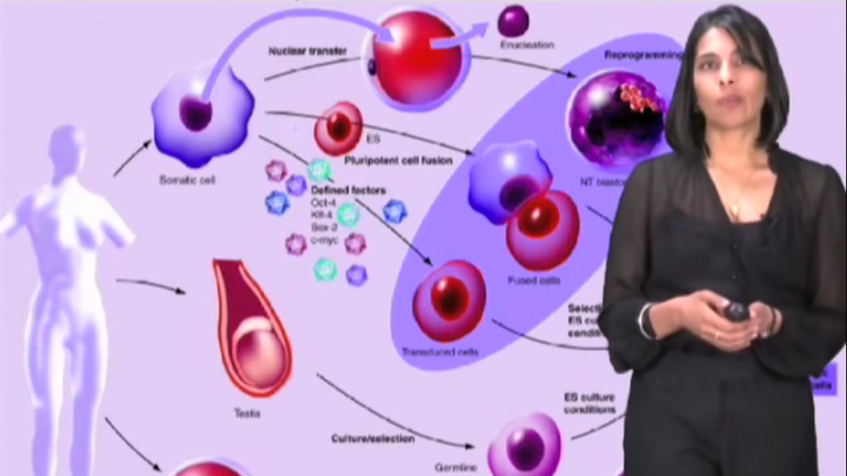
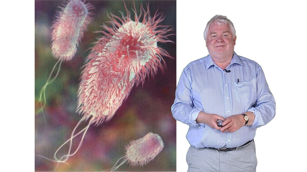
More Talks in Bioengineering

  • Sangeeta Bhatia Part 1: Engineering Tissue Replacements
    Tissue Engineering
  • Kristala L. J. Prather
    Introduction to Synthetic Biology and Metabolic Engineering
  • William Shih
    Nanofabrication via DNA Origami
  • Advancing the Treatment of Retinal Diseases
    Advancing the Treatment of Retinal Diseases

Reader Interactions

Leave a Reply Cancel reply

Your email address will not be published. Required fields are marked *

Primary Sidebar

Like our Website?

You'll love our newsletter...

  • Sign up for:
    • Exclusive iBiology content
    • 10 Must See Biology Videos
    • Talks by 20+ Nobel Winners
    • Our young Scientist Survival Toolkit
    • Talks by trailblazing Women in Biology
    • Updates on exciting iBiology projects in development
    Tyler Allen
  • This field is for validation purposes and should be left unchanged.

Privacy Policy

Help us keep bringing the world’s best biology to you!

Footer

Funders

National Science Foundation: NSF
Lasker Foundation
NIGMS

Partners

EMBL
EMBO
HHMI
NRMN
UCSF

Start Here

  • Talks for Everyone
  • Talks for Students
  • Talks for Research
  • Talks for Educators

Explore

  • Explore
  • All Playlists
  • All Speakers
  • All Talks

Talks By Topic

  • Biochemistry
  • Bioengineering
  • Biophysics
  • Cell Biology
  • Development and Stem Cells
  • Ecology
  • Genetics and Gene Regulation
  • Human Disease
  • Immunology
  • Microbiology
  • Neuroscience
  • Plant Biology
  • Techniques

Talks by Series

  • Bench to Bedside
  • Famous Discoveries
  • Great Questions
  • Share Your Research Series

Career

  • Professional Development
  • Career Exploration
  • NRMN Resources
  • Biomedical Workforce

Courses

  • Microscopy Series
  • Short Microscopy Series
  • Open edX Courses
  • Cell Biology Flipped Course
  • Engineering Life Flipped Course
  • Evolution Flipped Course

Educator

  • Educator Registration
  • Educator Resources
  • Log In

About Us

  • About Us
  • iBiology Team
  • Wonder Collaborative
  • Contact Us
  • Mission
  • Privacy Policy
  • SCL Financial Conflict of Interest Policy

This material is based upon work supported by the National Science Foundation and the National Institute of General Medical Sciences under Grant No. 2122350 and 1 R25 GM139147. Any opinion, finding, conclusion, or recommendation expressed in these videos are solely those of the speakers and do not necessarily represent the views of the Science Communication Lab/iBiology, the National Science Foundation, the National Institutes of Health, or other Science Communication Lab funders.

© 2022 - 2006 iBiology · All content under CC BY-NC-ND 3.0 license · Privacy Policy · Terms of Use · Usage Policy
 

Power by iBiology