• Skip to primary navigation
  • Skip to main content
  • Skip to primary sidebar
  • Skip to footer

iBiology

Bringing the World's Best Biology to You

  • Start Here
    • Explore iBiology
    • All Playlists
    • All Speakers
    • All Talks
    • What’s new at iBiology?
  • Research Talks
    • Talks by Topic
      • Biochemistry
      • Bioengineering
      • Biophysics
      • Cell Biology
      • Development and Stem Cells
      • Ecology
      • Evolution
      • Genetics and Gene Regulation
      • Human Disease
      • Immunology
      • Microbiology
      • Neuroscience
      • Plant Biology
      • Techniques
      • Archive
    • Talks by Series
      • Bench to Bedside
      • Famous Discoveries
      • Great Unanswered Questions
      • Young Scientist Series
  • Stories
    • Background to Breakthrough
    • Interviews and Profiles
    • Science and Society
  • Courses
  • Careers
    • Professional Development Talks
    • Professional Development Courses
    • Career Exploration
    • NRMN Resources
    • Biomedical Workforce
  • Educator
  • About
    • Mission
    • iBiology Team
    • Board of Directors
    • Make a Donation
    • iBiology Funders and Partnerships
    • Contact Us
Home » Courses » Microscopy Series » Fluorescence Microscopy

Förster Resonance Energy Transfer (FRET) Microscopy

  • Duration: 36:10
  • Downloads
    • Hi-Res
    • Low-Res
  • Subtitles
    • English
  • Transcript

00:00:12.06 In this seminar, I'm going to elaborate on how to image
00:00:15.10 molecular interactions in cells by using fluorescence
00:00:18.22 resonance energy transfer. So the way this seminar is set up is
00:00:24.00 as follows. I will start off with the principles of fluorescence
00:00:27.06 resonance energy transfer. I will then discuss the relevant
00:00:30.24 parameters that are important to understand to measure
00:00:34.08 specific molecular interactions. I'm going to discuss shortly
00:00:39.08 good fluorescent protein pairs to measure energy transfer
00:00:43.03 for every interaction. And then I'm going to discuss approaches
00:00:47.28 to actually image FRET with a microscope. And there's a specific
00:00:52.00 order over here, where I start off with the least quantitative,
00:00:55.05 but the easiest way of measuring, and as we move on, it becomes
00:00:58.09 more complicated as we get more quantitative information
00:01:00.21 about molecular interactions in cells.
00:01:03.08 So the idea of using fluorescence resonance energy transfer
00:01:07.07 to measure molecular interactions is based on detecting
00:01:11.02 coincidence of molecules. Normally what you do when you want to
00:01:17.09 detect interactions of molecules in let's say, a biochemical
00:01:19.25 experiment, you pull down one of the molecules and you look what
00:01:23.15 comes down. So it's kind of a direct measure of interaction.
00:01:26.02 In this case, we basically look at interaction inferring interaction
00:01:29.26 by coincidence in space. Now you can do that with a microscope.
00:01:33.27 And the problem with a normal wide-field microscope is that
00:01:38.29 in a way, the diffraction limits are observable elements.
00:01:42.23 So a typical volume element that you can resolve with a wide-field
00:01:46.12 microscope is in the order of a femtometer, which corresponds to
00:01:49.23 approximately a micron cubed. Of course the entities that we're
00:01:54.13 detecting, or the entities we want to know if they interact
00:01:56.23 have a way smaller volume, on the order of zeptometer,
00:02:00.10 on the order of 10^-22. So we have several orders of magnitude
00:02:04.21 difference in these scales. Now you can use colocalization
00:02:09.09 to infer interaction, but the probability that you have
00:02:13.28 an interaction when you see colocalization is very low.
00:02:17.09 So how can we improve it and how can we use FRET
00:02:19.17 to actually decrease this detection volume?
00:02:23.17 So, first let me discuss what FRET really is.
00:02:27.16 So, fluorescence resonance energy transfer is a non-radiative
00:02:31.08 transfer, and the word "nonradiative" is important. It's not
00:02:34.13 the trivial emission of a photon, but a reabsorption by the acceptor.
00:02:39.18 It's a dipole-dipole coupling mechanism. So it's a non-radiative
00:02:42.26 transfer of energy between nearby fluorophores.
00:02:45.16 Now, if you normally excite a donor, let's say with blue light,
00:02:50.08 in this case it's a GFP. It will very quickly relax from a high excited
00:02:54.26 state by interconversion or preparative relaxation to the first electron
00:02:59.05 excited state. From there it can do several things, it can go back to the
00:03:03.03 ground state by nonradiative decay interconversion. Or
00:03:07.02 it can emit a photon. If you have a coupling with an acceptor,
00:03:13.03 dipole-dipole coupling, then you have an extra channel
00:03:16.14 of nonradiative decay with shorter state lifetimes. So it means that
00:03:22.06 the acceptor -- sorry, the donor, will actually emit less light.
00:03:25.20 So you get a quenching of the donor when FRET occurs.
00:03:29.03 At the same time, the acceptor gets excited by this process.
00:03:34.21 Again, it's not the absorption of a photon, it's a dipole-dipole coupling
00:03:38.06 and it gets excited, and will then start emitting fluorescence.
00:03:41.23 And so you get basically emission from the acceptor
00:03:46.23 because of this process. So what we do is we cannot directly
00:03:51.04 measure FRET, it's not a direct observable, but we can
00:03:55.06 infer FRET from the change in photophysical properties
00:03:58.22 or the emission of the donor or the acceptor. So here are
00:04:05.04 a few relevant parameters that you can use to quantify FRET. One of them is actually the FRET efficiency. And the FRET efficiency
00:04:15.22 is basically the number of excited donors that transfer
00:04:19.21 the energy to the acceptor, divided by the number of photons
00:04:24.01 absorbed by the donor. This amounts of course to the number of
00:04:29.29 excited donors. So it's basically a fraction of donors that
00:04:34.13 transfer the energy to the acceptor. You can also put this in a
00:04:39.04 language of rates, these are transfer rates, seconds minus one.
00:04:42.21 So here we have basically the ratio between the transfer
00:04:46.22 rate divided by the total rate of exciting the donor.
00:04:51.29 Which is the transfer rate, again, plus the sum of
00:04:55.20 non-radiative decay down to the ground state and
00:04:57.24 radiative decay to the ground state, or transition to the ground
00:05:00.19 state. The efficiency can be shown to be equal to this ratio
00:05:06.06 where you see two parameters. One is the Forster radius,
00:05:12.16 or zero -- it's an important parameter, this represents the distance
00:05:16.23 at which the efficiency is 50%, so half the excited donor
00:05:20.03 molecules transfer to the acceptor. And this is typically in the order
00:05:23.28 of nanometers. So you get this process going on in nanometer range.
00:05:29.18 It also appears over here and here we have basically the distance
00:05:33.21 between the donor and acceptor. And you can see it's
00:05:37.01 r^6 dependence, which makes it very steep dependence.
00:05:40.10 So the efficiency is a way of measuring distances between the
00:05:46.24 donor and acceptor. So here I have plotted the FRET efficiency
00:05:53.03 as a function of distance between the donor and acceptor
00:05:56.06 in units of the Forster Radius. So if you have a Forster radius
00:06:00.18 or a radius of 1, then you must have 50% energy transfer shown over here.
00:06:06.14 The point is as follows, if you have molecules that do not
00:06:12.05 interact in solution, the average distance is so large that you cannot get
00:06:17.24 energy transfer. To give you an example, if you have a
00:06:21.05 one micromolar solution, the average distance between
00:06:24.07 molecules is in the order of 100 nanometers, which is about
00:06:27.21 20 units on this scale, which is way off to the right.
00:06:31.06 So you won't get energy transfer. However, if you go to concentration
00:06:35.02 of 1 millimolar, the average distance becomes something
00:06:38.02 like 10 nanometers, and we're getting close to this point over
00:06:41.14 here. However, when we express proteins in cells, we are
00:06:46.13 typically on the order of 1-10 micromolar concentration,
00:06:50.21 and in solution that should not be a problem. So we're way
00:06:53.12 off here, so we don't get this trivial FRET process.
00:06:56.08 Which is due to the concentration and average molecules.
00:06:59.26 Because of the steep distance dependence, you basically have a
00:07:04.08 situation where no interaction doesn't give you FRET,
00:07:06.16 and interacting molecules give you FRET. So these are our
00:07:14.18 parameters that determine our zero. And over here, the first
00:07:20.13 factor called kappa squared is actually a factor that is a geometric factor.
00:07:25.15 It is defined by the orientation of transition moments,
00:07:29.23 which are transition dipoles. When two molecules have
00:07:34.14 transition moments aligned, the process of transfer becomes
00:07:40.04 very efficient, they have a factor of 4. However, when they're
00:07:43.19 perpendicular, that factor is basically 0. So you can have a situation
00:07:47.08 where two chromophores are seeming proximal, but they're at
00:07:52.00 right angles with the transition moments, so you don't get FRET.
00:07:53.21 Now in general, that factor's stated to be 2/3, where you basically
00:08:01.17 average over all orientations. This means very floppy fluorophores
00:08:04.02 that move in all directions. Basically in the time of transfer,
00:08:07.09 you sample all orientations. Can be shown that this factor
00:08:11.26 is 2/3. Unfortunately, for fluorescent proteins, the chromophores
00:08:17.27 are embedded in the barrel and is quite rigid. And a reorientation
00:08:21.04 of the barrel is rather slow on a time scale of transfer.
00:08:24.29 Which means we can't actually do this dynamic averaging
00:08:28.19 for this kind of static averaging that we get. And so that
00:08:32.14 poses a problem, and that will actually inhibit us from using
00:08:36.19 the efficiency to calculate distance between molecules.
00:08:41.01 However, still a change in efficiency in a complex will tell us
00:08:45.08 if there are, for example, a conformational change going on.
00:08:48.21 If you put it to 2/3, we can actually compare different fluorescent
00:08:55.09 protein pairs, in terms of the efficiency of transfer.
00:08:58.03 I just make it a constant. The second parameter over here, is a
00:09:04.24 refractive index, which for let's say cytoplasm, is set to 1.4.
00:09:09.16 So that's more or less a constant, we don't worry about
00:09:12.03 it too much. This factor over here is the overlap integral.
00:09:19.22 Which represents the resonance principle, which is overlap between
00:09:25.01 the emission of the donor and the absorption of the acceptor.
00:09:30.20 It says how much the actual energy levels are matched. The more they're
00:09:34.18 matched, the better you get the transfer. And it's defined by this integral
00:09:39.02 shown over here, which shows again the emission spectrum,
00:09:41.24 the absorption spectrum. So two things to consider here,
00:09:47.28 the extinction coefficient of the acceptor is an important
00:09:53.25 parameter. The higher it is, the more efficient the transfer.
00:09:56.20 So you want to have molecules with the high extinction
00:10:01.05 coefficient, to increase your R0. It represents the ability
00:10:05.20 of the molecule to absorb photons. The other factor that's
00:10:09.29 important is this lambda to the 4th. So basically, the overlap
00:10:14.06 integral becomes higher when you move to the red part of the
00:10:17.21 spectrum, which means when you're using fluorescent proteins
00:10:20.02 that are more in the red part of the spectrum, the overlap
00:10:23.03 integral becomes larger. And you get a bigger R0.
00:10:28.21 Quantum yields, given over here, quantum yield of the donor.
00:10:35.17 The more photons that can be emitted from the donor
00:10:39.09 when it's in an excited state, the better the transfer process.
00:10:41.29 And this can be maximally 1. So here are some R0 values
00:10:47.12 that I've done for several fluorescent proteins that are available
00:10:51.26 at the moment. And I've started off by representing the R0
00:10:55.28 for the classical pair, the cyan fluorescent protein and the yellow
00:10:59.17 fluorescent protein. This pair was used a lot in the past because
00:11:02.29 we didn't have a choice for other fluorescent protein pairs.
00:11:06.11 The R0 is quite moderate, so it's close to 5 nm, but nowadays
00:11:12.08 because we can have more red emitting fluorophores, we can
00:11:16.09 actually increase our R0 to better detect interactions.
00:11:19.03 Also, we have better cyan fluorescent proteins, for example,
00:11:23.14 that increase quantum yield, one of the parameters that was
00:11:25.24 important for our R0, and therefore increase the R0.
00:11:29.06 So for example, this cerulean is a variant of cyan fluorescent protein,
00:11:32.26 with the acceptor citrine, which is a variant of the yellow
00:11:35.13 fluorescent protein, already has an R0 of 5.3. Now if we use,
00:11:40.24 for example, mCitrine as a donor now instead of an acceptor,
00:11:44.05 we have an orange fluorescent protein as an acceptor, we go now
00:11:47.25 to almost 5.5 nm. If we use citrine with a red fluorescent protein
00:11:51.26 as acceptor, we can go close to 6 nm. These pairs are typically
00:11:58.23 pairs that we use at the moment to detect FRET, especially
00:12:01.05 this one over here, the citrine and cherry. They have very good
00:12:05.14 folding properties, and therefore it's very good to measure
00:12:08.11 interactions in cells, with an R0 close to 6 nm.
00:12:12.09 So back to our coincidence detection, if you just measure
00:12:16.29 coincidence of molecules by colocalization using a microscope,
00:12:20.16 our detectable volume element is way too large compared
00:12:24.12 to our volume that we're detecting. If you now look at the
00:12:29.18 coincidence of molecules using FRET, we're going to a volume
00:12:32.27 that is in the same order as the volume of the molecules that
00:12:36.21 we want to detect. So we're in this sub-zeptometer domain or
00:12:40.23 sub-zeptometer scale for an R0, for example, of 4.6 nm.
00:12:45.11 Now, important point to make here, FRET is not a technique
00:12:49.16 to improve resolution. It's not like a super resolution technique.
00:12:52.07 It gives you a signal about how many molecules in a volumable element
00:12:57.17 are actually interacting, proportional to the amount of molecules
00:13:00.08 that are interacting. That's an important point to make. So no
00:13:03.06 increase in resolution. So what do we actually measure
00:13:07.29 when we quantify FRET? So, different approaches, but in fact
00:13:12.11 we measure apparent efficiency. And this measured efficiency,
00:13:15.11 equals the real efficiency, transfer efficiency, as only defined
00:13:19.26 for the complex. So there where you have FRET.
00:13:24.16 And that is actually a geometric parameter, it gives
00:13:28.00 information about distances and angles. In a way it's
00:13:31.07 a measure of the conformation of the molecule. The apparent efficiency
00:13:38.03 is also proportional to the fraction of interacting molecules
00:13:41.29 at each volumable element. And that's really an image, so here
00:13:45.23 we can look at reaction progression. So how many molecules
00:13:50.14 are interacting at this specific volume element that we have
00:13:56.00 as compared to over here? This is actually a biologically relevant
00:14:01.00 parameter, which is a local parameter which gives us a real
00:14:05.23 map. Whereas the efficiency is not a local parameter, it's actually
00:14:13.09 global parameter, which is only defined by properties of the molecule.
00:14:16.24 I'll come back to that property. So before I elaborate on the
00:14:25.06 different approaches to measure FRET in a microscope,
00:14:27.15 there's one important point to consider, which is the shape of
00:14:32.04 the spectrum. So when you look at absorption spectra,
00:14:35.29 there's always a tail toward the blue part of the spectrum,
00:14:40.04 and are steep at the red part of the spectrum. That is typical.
00:14:45.04 When you look at the emission spectrum, the fluorescence emission
00:14:49.13 spectra, they do exactly the opposite. They're very steep
00:14:52.23 at the blue part of the spectrum, but they tail towards the red.
00:14:58.03 And that's why we can specifically excite the acceptor, you can see
00:15:08.18 when we excite the acceptor we don't don't excite the donor, but
00:15:11.12 we cannot excite the donor without exciting the acceptor.
00:15:15.13 And similarly, we can detect the donor without detecting
00:15:21.18 the acceptor, but not specifically detect the acceptor without
00:15:27.23 detecting the donor. So these two specific excitation of the
00:15:34.16 acceptor, specific detection of the donor, is relevant to what I'm going
00:15:38.09 to elaborate on when we talk about the measurements to get
00:15:42.20 FRET -- to a FRET measurement in a microscope.
00:15:45.27 So this is the most straight-forward and simple approach
00:15:50.14 that has been used a lot in the past. It's purely based on the
00:15:56.11 fact that if you have FRET, you quench the donor, but you
00:15:59.28 increase the intensity of the acceptor by sensitized emission.
00:16:03.00 So you excite the acceptor by this process. So what you do is
00:16:06.24 excite the donor and you measure the donor image, so the
00:16:14.09 donor emission image. And you measure an acceptor emission
00:16:19.12 by exciting the donor. And you see you have two images,
00:16:23.23 which you ratio in this way. So donor excitation and acceptor
00:16:26.27 emission, donor excitation and donor emission.
00:16:30.18 Now because we have the problem that we still have
00:16:34.09 the red excitation of the acceptor, and we have bleed through
00:16:37.28 of the donor, this only works when a donor and acceptor
00:16:42.18 are in the same molecule, so in the same polypeptide.
00:16:46.28 You need to keep the stoichiometry of donor and acceptor
00:16:53.06 constant in each pixel. So this specifically works, for example,
00:16:57.25 for sensors like a chameleon, that can measure a change
00:17:01.04 in a physiological parameter like calcium, but can also
00:17:03.25 measure phosphorylation. And again, I'll give an example
00:17:05.09 of that. So here we have a construct which you can measure
00:17:11.16 in a ratiometric way. So it's epidermal growth factor receptor, its
00:17:15.05 name is ErbB-1, where we have now in one chain the donor
00:17:20.28 CFP, we have a PTB domain, specifically recognizing phosphotyrosines,
00:17:25.16 and we have yellow fluorescent protein as an acceptor.
00:17:28.24 Realize that in whatever conformation that this might already have
00:17:33.14 basal FRET, you only see a change in the configuration. So a
00:17:37.26 change in the FRET efficiency. So this measurement gives you in a way
00:17:41.18 a relative measure of the conformation of the molecule.
00:17:46.12 So it's very easily implemented. Can do it on very different
00:17:51.16 types of setups, like confocal setups or wide-field imaging,
00:17:54.08 with the right filter sets, it's very fast because you just need to
00:17:56.26 acquire two images. It's not quantitative, you can only measure
00:17:59.29 differences in states. And you need to keep the stoichiometry of donor
00:18:04.05 and acceptor constant. Which basically means that they have to be the
00:18:07.28 same construct. Here is an example of how such an experiment
00:18:13.13 looks like. So we have expressed this construct in Cos7
00:18:16.18 cells. You see the fluorescence of YFP over here, where you see the addition of
00:18:20.18 the receptor on membranes and also on vesicles inside.
00:18:23.17 And here we measure what happens when you add EGF, you actually
00:18:26.23 activate the receptor. The blue represents the phosphorylated
00:18:29.22 receptor. So you see basically there's an area inside the cytoplasm
00:18:31.29 that shows active receptor, but there's also an area inside
00:18:35.20 the cytoplasm where it's an inactive receptor, where it becomes
00:18:38.08 inactive. So here we can see at the end of the sequence,
00:18:42.14 we can actually inhibit the kinase activity and the whole thing shoots
00:18:45.19 back up because we inhibit the kinase activity which cannot then
00:18:49.24 self-phosphorylate or auto-phosphorylate. So let's move
00:18:53.22 one step further and try to use a measurement now which is slightly
00:18:59.03 more quantitative than this approach. Where we can actually use the donor
00:19:02.09 and the acceptor on separate proteins. So this is the approach of
00:19:06.26 sensitized emission. Now in an ideal situation, if you could
00:19:11.22 excite the donor specifically without exciting the acceptor,
00:19:16.28 and we would monitor the fluorescence of the acceptor and we would only
00:19:20.00 get emission from the acceptor when there is energy transfer.
00:19:23.25 So we would basically make an image where we excite the donor
00:19:27.19 and detect the acceptor. The problem of course is that
00:19:33.00 we're directly exciting the acceptor and we have bleed
00:19:41.23 through of the donor in the acceptor channel. So the image
00:19:48.01 where you excite the donor and you look at the acceptor,
00:19:52.04 doesn't equate to the sensitized emission. We have contamination
00:19:55.11 from direct excitation and bleed through. Now before I
00:20:00.12 go a little bit further, look at the spectra. We cannot really look
00:20:06.15 in our example where we have donor and acceptor. We cannot
00:20:09.27 really determine how much acceptor goes through.
00:20:12.28 However, what we can do is we can measure the amount
00:20:16.20 accepted when excited directly at its peak. Because there we don't
00:20:19.09 excite the donor, so that's very specific. So if we somehow
00:20:22.27 know, let's say, the ratio between these two, which is
00:20:26.23 a fixed number. Then we could actually determine by measuring
00:20:30.21 here how much is there. Exactly the same situation with the
00:20:34.23 donor bleed through. We cannot measure in a sample where we have
00:20:39.00 donor and acceptor, because we have the emission of the acceptor.
00:20:44.00 But we can measure the donor specifically, so again we know the
00:20:49.13 relationship is the ratio, that by measuring here we can determine
00:20:53.09 how much is there. As long as the spectra, the shape, is invariant.
00:20:57.01 So how do we do this correction? How do we determine
00:21:02.22 these correction factors? We take the sample with the donor alone
00:21:07.25 and determine basically the ratio between this and this, and we take
00:21:14.16 the sample with the acceptor alone and we take the ratio between this
00:21:16.27 and this. And thereby, by measuring in a sample where we have donor
00:21:22.06 and acceptor, by exciting the acceptor, we can determine how much we
00:21:26.01 directly excite the acceptor. So this is how the experiment goes.
00:21:32.23 We express the donor, in this case, we're going to correct for bleed through.
00:21:37.07 We excite the donor, we just now have a donor spectrum,
00:21:41.16 because there's no acceptor, and measure at emission
00:21:46.07 of the acceptor. In other words, to correct in a sample where we have donor
00:21:53.15 and acceptor, we need to know how this relates to this
00:21:58.15 intensity. And so we measure at the peak of the donor
00:22:03.23 and now, by this ratio, we have to scale our correction factor
00:22:09.06 by which we need to correct the image where we excite the donor
00:22:14.06 and measure the donor, in order to subtract it from the
00:22:18.28 sensitized emission, or the FRET channel. Very similar
00:22:25.18 principle for the correction of direct excitation.
00:22:28.01 We take now a sample which now contains the acceptor
00:22:31.16 alone. In the sample where we have donor and acceptor,
00:22:37.17 we cannot determine how much is there because it's also the donor.
00:22:41.04 So we measure in a sample where we have donor and
00:22:48.02 acceptor, this part so we know how much is there. So we need to
00:22:52.08 obtain the ratio, and it's exactly the same situation. So
00:22:55.18 basically get the scale up correction factor, where we take
00:22:59.20 image with the acceptor alone and we excite the donor,
00:23:02.17 that's where we have the direct excitation, measure the acceptor,
00:23:08.00 divided by the image of direct excitation of the acceptor
00:23:11.05 and measurement of the acceptor. So then the sensitized
00:23:15.16 emission is built up as follows. We have our donor excitation and
00:23:22.06 acceptor emission, in the ideal world, that would be the
00:23:26.20 sensitized emission, however we have the contributions
00:23:29.00 from the donor bleed through and the acceptor direct excitation.
00:23:35.04 Because you can measure the donor in a sample that contains both
00:23:40.14 donor and acceptor, specifically at the donor wavelength,
00:23:42.19 you get a measure of this bleed through which you need to correct
00:23:46.28 by this scalar factor. Exactly the same situation for direct
00:23:51.03 excitation of the acceptor. So we have basically three images,
00:23:56.07 we take the donor excitation/acceptor emission, donor
00:24:00.23 excitation/donor emission, acceptor excitation/acceptor emission.
00:24:04.26 And then in a separate experiment, we determine these two
00:24:07.28 scalar factors. And we divide this by the acceptor intensity,
00:24:14.27 so exciting the acceptor and acceptor emission, and we get the measure
00:24:18.27 of the apparent efficiency that is proportional to the real efficiency
00:24:22.26 and the fraction of interacting molecules. So this is very easy
00:24:29.03 to implement on standard microscopes, you can do it in a
00:24:31.09 confocal microscope, you can do it in a wide-field microscope with
00:24:34.22 appropriate filter sets. It's rather fast, because you can switch
00:24:39.19 your filters very quickly on a filter wheel or on a confocal microscope
00:24:43.15 you can almost do it simultaneously. Or you can do it
00:24:45.24 simultaneously. It's semi-quantitative, because you get something that's proportional
00:24:50.07 to the relative concentration of interacting molecules.
00:24:53.12 The problem here is of course depends on this external calibration,
00:24:57.05 so the get the scalar factors, where you need the sample with donor
00:25:00.11 alone and acceptor alone, which makes it also very sensitive to noise.
00:25:04.27 And one important other property that you need to have
00:25:07.08 is the spectra basically being invariant to the environment,
00:25:11.27 so they don't change their shape dependent on the environment.
00:25:15.01 Like for example, if it's a lipid environment or a cytoplasmic
00:25:18.01 environment. That is the case for fluorescent proteins
00:25:21.11 fortunately, because the chromophore is encased in the
00:25:23.29 barrels. The environment is defined by the barrels.
00:25:26.04 So an example here, again we use the same system,
00:25:31.14 we have epidermal growth factor receptor now attached with a
00:25:35.12 donor. Now we have the separate expression of this PTB
00:25:39.21 domain that recognizes phosphotyrosine tagged with the acceptor.
00:25:42.24 Because we make the corrections, we can have them in separate
00:25:46.13 constructs. We don't need to attach them. So here is basically
00:25:50.00 the role that represents the distribution in space of the
00:25:54.15 receptor, you have the PTB domain, and here we have
00:25:57.18 the apparent efficiency. Now this is a very simple experiment,
00:26:00.25 basically no stimulation you can see this is already active
00:26:03.18 receptor. There's already interaction over here. When we add
00:26:06.16 EGF, you get an increase of interaction that more receptors
00:26:09.25 activated. When we add an inhibitor of the kinase, a short
00:26:15.29 time it still stays on because the phosphatase takes some time to
00:26:19.04 actually phosphorylate the receptor, but at longer times you actually
00:26:21.13 lose that interaction again. So this is the third intensity based
00:26:29.15 approach that I will describe. From the intensity based approaches
00:26:32.28 this is the most quantitative. But it has a big disadvantage
00:26:36.04 as compared to the previous methods I was describing.
00:26:38.20 You can only use it in fixed cells, which is very difficult to do in
00:26:42.10 live systems. The advantage of this approach is that it is
00:26:46.13 very robust and is quite quantitative. So how does this work?
00:26:51.26 It's as follows. We excite the donor and then look at the
00:26:58.12 emission of the donor. If FRET goes on, the donor should be
00:27:03.02 quenched. And so there's less emission from it because it's
00:27:06.02 actual channel of nonradiative decay. What we would like to know
00:27:13.16 is what is the donor intensity in the absence of acceptor?
00:27:17.07 Using that it is very easy to calculate the efficiency.
00:27:22.17 Now we cannot do a separate experiment where we measure the donor
00:27:27.07 alone, because it would be a completely different configuration,
00:27:28.28 and different concentration of molecules and so on.
00:27:30.28 So what we do is the following. We excite the acceptor
00:27:34.19 and you can do highly specific, and basically excite until it's
00:27:37.25 photobleached completely. So we destroyed the acceptor antennae.
00:27:41.20 And then after that, we remeasure the donor. And then
00:27:45.23 the donor will unquench and the intensity will go up,
00:27:49.01 and you have the situation in the absence of the acceptor.
00:27:55.00 Of course in a live cell situation, where things move very fast, this is not possible. You'll change the interactions, you'll change
00:28:02.01 where molecules are, and this will not be a good measure anymore.
00:28:05.03 That's why you want to do this in fixed cells. Now, the apparent
00:28:09.09 efficiency is basically 1 minus the donor in the situation where you have the
00:28:14.10 acceptor that's quenched, and then the donor in the situation
00:28:20.07 where you have photobleached the acceptor. This is what it looks
00:28:25.01 like in a real experiment. Here again we have the same system
00:28:30.06 just to make this comparison. So again we have epidermal
00:28:32.25 growth factor receptor, and in this case, we look actually at
00:28:35.20 phosphorylation of the tyrosines by looking at an antibody
00:28:38.24 that has a chemical acceptor, a small tag as an acceptor.
00:28:45.11 This is in fixed cells, before photobleaching or acceptor
00:28:48.15 photobleaching. It's best done in fixed cells, it's difficult in live
00:28:51.12 cells. And we basically have incubated with this antibody.
00:28:55.00 Now the point here is that this antibody is not specific
00:28:57.14 for EGFR phosphotyrosines, it also recognizes any
00:29:01.09 phosphotyrosine. However, because we measured the
00:29:04.12 proximity of this antibody to this molecule with FRET,
00:29:07.01 you get a highly specific signal for the phosphorylation
00:29:10.21 of the receptor. Specifically for that receptor. So here you have
00:29:15.10 basically the donor alone, that's the distribution of receptor,
00:29:18.03 here below is the acceptor distribution, it's the antibody.
00:29:21.21 It's there where you have phosphorylation. And then
00:29:24.15 you photobleach in this rectangle the acceptor, you can see it
00:29:30.12 disappeared over here. We did this in a confocal microscope,
00:29:32.25 so we just took an area, a region of interest, and photobleached it
00:29:35.21 over there. This becomes in the reference version.
00:29:39.00 And what you see is in the donor, you actually see it increase
00:29:40.28 in the intensity there where you had FRET, where you compare this
00:29:44.14 situation over here, for example, to the situation over here.
00:29:47.08 It's also very nicely seen in this image where you have
00:29:51.01 the difference between these two, and so you see basically
00:29:54.25 unquenching versus the reference version, where there's hardly
00:29:56.29 anything going on. Now if you take 1 minus this image
00:30:01.20 divided by that image, you get the apparent FRET efficiency,
00:30:05.03 which shows that you have active receptor mostly
00:30:08.03 at the plasma membrane and very little active receptor
00:30:12.03 on this internal vesicle. So basically it's dephosphorylated
00:30:17.00 in this compartment. So this approach is very easily implemented,
00:30:21.24 it's highly robust. It's actually used as a standard to prove
00:30:26.14 that FRET is going on. It's very slow, and that is the biggest disadvantage.
00:30:32.05 It's not suitable for live cell imaging. There's possibly a solution
00:30:35.21 here by using photochromic dyes or switchable dyes that you can
00:30:39.12 switch back and forth, on and off, to do it in live cells.
00:30:42.02 I'm not going to discuss that. It's semi-quantitative, but you get
00:30:46.26 something that's proportional to the fraction of complex
00:30:49.06 true efficiency. So in that sense, it's the most quantitative
00:30:53.06 in terms of the intensity based methods. And you don't need an
00:30:56.10 external calibration, which was the case for sensitized emission
00:30:59.09 measurements. You have an internal control by this bleaching.
00:31:02.19 So one more example that I'll show over here, just to show
00:31:08.13 you that you can use this approach to also for example do a
00:31:11.28 three dimensional map of interaction. In this case, we looked
00:31:14.24 at interaction between epidermal growth factor and a
00:31:18.24 phosphatase called PTP1B that's on the surface of the ER.
00:31:22.07 And we used a specific tracking mutant that has a stable
00:31:25.25 interaction with its substrate. So we wanted to know where
00:31:27.29 does the phosphatase actually act on epidermal growth factor.
00:31:31.08 So what you do is you take the donor stacks, so you take a
00:31:36.10 complete stack to obtain a three dimensional distribution
00:31:38.28 of your donor. You then photobleach the acceptor by just
00:31:42.23 scanning over one plane, because the dose effect of photobleaching
00:31:45.20 just stays in one place, in at least one photon approaches.
00:31:49.01 You photobleach the acceptor completely, then retake
00:31:52.15 the three dimensional stack and you just take 1 minus the
00:31:55.07 ratio of these two images, and you obtain the apparent
00:31:59.01 efficiency. And now you can see in this green area basically where this
00:32:02.23 interaction takes place. You can clearly see that this is where the
00:32:05.13 receptor gets dephosphorylated, basically inside the cell.
00:32:10.15 So this is the last approach I'm going to describe. And I'm
00:32:16.23 going to elaborate more on the second seminar, which deals
00:32:19.27 specifically with it, because it's the most quantitative
00:32:21.24 approach, but also involves a little bit more, I'd say, technical
00:32:25.20 equipment. More elaborate equipment, but also more
00:32:31.20 elaborate analysis methods. And it's worth discussing it separately.
00:32:35.11 The major strength really is quantification. So measuring
00:32:41.00 FRET by fluorescence lifetime imaging microscopy, what we do here
00:32:44.01 is we measure the excited state lifetime of the donor.
00:32:46.17 So you excite the donor and you measure the donor, which you can do
00:32:52.04 specifically, not without seeing the acceptor. And instead of
00:32:55.28 measuring the intensity, what we do is we measure the
00:32:59.14 excited state decay as a function of time.
00:33:04.14 And if you have FRET, then you have an extra channel of
00:33:07.10 non-radiated decay. So you depopulate the excited state
00:33:09.27 faster, and that means you will always get a shorter
00:33:12.26 or a more rapid decay, which means a shorter lifetime.
00:33:17.27 Now just to give you a flavor of what it looks like, I just have an example
00:33:22.13 here, which I will come back to in my second seminar.
00:33:24.18 Where we looked at interaction between Ras, which is
00:33:28.24 central in signal transduction, which has the donor molecule
00:33:32.17 Citrine attached to it. And this molecule called PDEd, which is
00:33:36.20 GDI-like solubilizing factor, with a Cherry attached to it.
00:33:41.04 We're interested in this interaction because it was of importance
00:33:44.12 to the spatial organization of Ras, and we need to know where this
00:33:47.23 interaction takes place inside cells. So we basically measured
00:33:51.09 FRET and we do this specifically by measuring the excited
00:33:53.27 state properties of the donor. Now what we obtain with FLIM
00:33:59.10 in a single experiment, is the true efficiency in the complex
00:34:05.21 which is a geometric parameter, with space variant.
00:34:10.00 It's only property of the complex, which allows us to say something about
00:34:14.21 the conformation. If you take off kappa squared, ignore kappa squared,
00:34:17.21 we can actually say that there is a 50% energy transfer
00:34:20.17 efficiency and approximately a transfer distance of 6 nm.
00:34:23.16 But that is very dangerous. More important, and that is really relevant
00:34:28.11 for biologists, in my opinion, is this parameter alpha, which is
00:34:33.21 the fraction of interacting molecules in each pixel or spatial
00:34:39.05 resolvable element. This represents reaction progression
00:34:42.16 where the interactions take place, and this is truly a map
00:34:45.07 in contrast to E, which is not a map, that's just a scalar.
00:34:49.14 It's a property of the complex, this is a property that varies as a function
00:34:53.29 of space. So here we get then the fraction, in our false color table
00:34:59.26 a fraction of molecules that are interacting. In this case, Ras
00:35:04.09 interacting with PDEdelta, and you can see right here that the plasma
00:35:07.18 membrane we do not find interaction. And at the golgi, we do not
00:35:10.12 find interaction. Whereas here you see interaction in the
00:35:12.29 cytoplasm. And this is highly relevant to couple let's say the state
00:35:16.27 of Ras to its interaction with PDEdelta.
00:35:25.06 So next time, I'm going to elaborate on this fluorescence
00:35:29.00 lifetime imagine microscopy, because it deserves a separate
00:35:31.25 discussion because it's the most quantitative approach
00:35:36.05 and allows you to quantitate the biology and better understand
00:35:40.08 how molecular reactions, for example, are important for spatial organization.

This Talk
Speaker: Philippe Bastiaens
Audience:
  • Researcher
Recorded: May 2012
More Talks in Microscopy Series
  • Philippe Bastiaens Fluorescence Lifetime Imaging Microscopy
    Fluorescence Lifetime Imaging Microscopy
  • Microscopy: Designing a Fluorescence Microscopy Experiment (Kurt Thorn
    Summary: Designing a Fluorescence Microscopy Experiment
  • Labeling Proteins with Fluorescent Probes (Timothy Mitchison)
    Labeling Proteins with Fluorescent Probes
All Talks in Microscopy Series
Share

Talk Overview

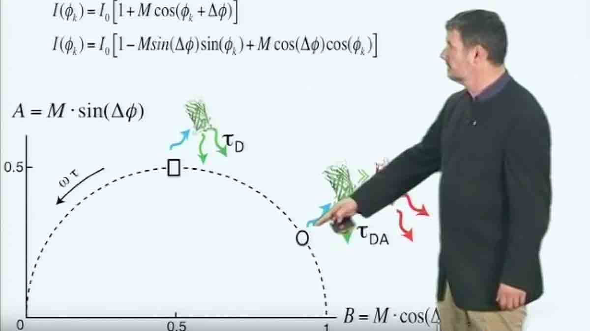
Förster Resonance Energy Transfer (FRET) microscopy is a technique that allows monitoring of interactions between dyes that occur on the nanometer scale. This sensitivity to small changes in distance and orientation make it a popular technique for building biosensors. Here, Philippe Bastiaens describes the physics behind FRET and how FRET can be measured with a microscope.

Questions

  1. FRET is
    1. Absorption by acceptor of fluorescence light emitted by the donor
    2. Nonradiative transfer of energy between nearby molecules with correctly oriented dipoles
    3. Quenching of fluorescence emitted by acceptor in the presence of donor molecules
    4. A directly observable physical phenomenon involving fluorescence
  2. The Förster distance is not a function of
    1. Orientation factor
    2. Refractive index
    3. Overlap between emission of donor and absorption of donor
    4. Distance between the two molecules
  3. Förster distances typical for fluorescent proteins are:
    1. 1-3 Angstrom
    2. 4-7 Angstrom
    3. 1-3 nm
    4. 4-7 nm
  4. FRET can be measured by ratio imaging when
    1. Donor and acceptor are part of the same molecule
    2. Donor and acceptor absorption and emission spectra are known
    3. There is no overlap in the excitation spectra of donor and acceptor
    4. There is no overlap in the emission spectra of donor and acceptor
  5. To estimate sensitized emission, one needs to correct for
    1. Donor emission at the acceptor emission wavelengths
    2. Acceptor excitation at the donor excitation wavelengths
    3. Nothing
    4. A and B
  6. FRET measurement by acceptor photobleaching is based on
    1. Quenching of the acceptor
    2. Movement of molecules during photobleaching
    3. Dequenching of the donor
  7. FRET
    1. Increases the lifetime of the donor
    2. Decreases the lifetime of the donor
    3. Increases the lifetime of the acceptor
    4. Decreases the lifetime of the acceptor

Answers

View Answers
  1. B
  2. D
  3. D
  4. A
  5. D
  6. C
  7. B

Speaker Bio

Philippe Bastiaens

Philippe Bastiaens

Philippe Bastiaens is Director of the Department of Systemic Cell Biology at the Max Planck Institute of Molecular Physiology and a Professor at the Technische Universitat Dortmund. Bastiaens and his colleagues have developed special fluorescence microscopy techniques such as FLIM and FRET, and use them to explore protein signaling pathways. Continue Reading

Playlist: Microscopy Series

  • Microscopy: Quantitative Analysis of Speckle Microscopy: Clare Waterman
    Measuring Dynamics: Fluorescent Speckle Microscopy
  • Philippe Bastiaens Fluorescence Lifetime Imaging Microscopy
    Fluorescence Lifetime Imaging Microscopy
  • Microscopy: Designing a Fluorescence Microscopy Experiment (Kurt Thorn
    Summary: Designing a Fluorescence Microscopy Experiment
  • Labeling Proteins with Fluorescent Probes (Timothy Mitchison)
    Labeling Proteins with Fluorescent Probes

Reader Interactions

Comments

  1. Tóth Benedek says

    May 9, 2018 at 10:27 am

    Dear Mr. Philippe,

    Why do I have to keep the stochiometry of donor and acceptor constant during ratio imaging?

    Sincerely, Tóth Benedek

    Reply

Leave a Reply Cancel reply

Your email address will not be published. Required fields are marked *

Primary Sidebar

Like our Website?

You'll love our newsletter...

  • Sign up for:
    • Exclusive iBiology content
    • 10 Must See Biology Videos
    • Talks by 20+ Nobel Winners
    • Our young Scientist Survival Toolkit
    • Talks by trailblazing Women in Biology
    • Updates on exciting iBiology projects in development
    Tyler Allen
  • This field is for validation purposes and should be left unchanged.

Privacy Policy

Help us keep bringing the world’s best biology to you!

Footer

Funders

NSF Logo
Lasker Logo
NIGMS Logo

Partners

Start Here

  • Talks for Everyone
  • Talks for Students
  • Talks for Research
  • Talks for Educators

Explore

  • Explore
  • All Playlists
  • All Speakers
  • All Talks

Talks By Topic

  • Biochemistry
  • Bioengineering
  • Biophysics
  • Cell Biology
  • Development and Stem Cells
  • Ecology
  • Genetics and Gene Regulation
  • Human Disease
  • Immunology
  • Microbiology
  • Neuroscience
  • Plant Biology
  • Techniques

Talks by Series

  • Bench to Bedside
  • Famous Discoveries
  • Great Questions
  • Share Your Research Series

Career

  • Professional Development
  • Career Exploration
  • NRMN Resources
  • Biomedical Workforce

Courses

  • Microscopy Series
  • Short Microscopy Series
  • Open edX Courses
  • Cell Biology Flipped Course
  • Engineering Life Flipped Course
  • Evolution Flipped Course

Educator

  • Educator Registration
  • Educator Resources
  • Log In

About Us

  • About Us
  • iBiology Team
  • Wonder Collaborative
  • Contact Us
  • Make a Donation
  • Mission
  • Privacy Policy

This material is based upon work supported by the National Science Foundation and the National Institute of General Medical Sciences under Grant No. MCB-1052331. Any opinion, finding, conclusion, or recommendation expressed in these videos are solely those of the speaker and do not necessarily represent the views of iBiology, the National Science Foundation, the National Institutes of Health, or other iBiology funders.

© 2021 - 2006 iBiology · All content under CC BY-NC-ND 3.0 license · Privacy Policy · Terms of Use · Usage Policy
 

Power by iBiology


This website uses cookies to remember you and improve your experience. To find out more see our Privacy Policy.Accept