• Skip to primary navigation
  • Skip to main content
  • Skip to primary sidebar
  • Skip to footer

iBiology

Bringing the World's Best Biology to You

  • Start Here
    • Explore iBiology
    • All Playlists
    • All Speakers
    • All Talks
    • What’s new at iBiology?
  • Research Talks
    • Talks by Topic
      • Biochemistry
      • Bioengineering
      • Biophysics
      • Cell Biology
      • Development and Stem Cells
      • Ecology
      • Evolution
      • Genetics and Gene Regulation
      • Human Disease
      • Immunology
      • Microbiology
      • Neuroscience
      • Plant Biology
      • Techniques
      • Archive
    • Talks by Series
      • Bench to Bedside
      • Famous Discoveries
      • Great Unanswered Questions
      • Microscopy Series
      • Share Your Research Series
  • Stories
    • Background to Breakthrough
    • Interviews and Profiles
    • Science and Society
  • Courses
  • Careers
    • Professional Development Talks
    • Professional Development Courses
    • Career Exploration
    • NRMN Resources
    • Biomedical Workforce
  • Educators
  • About
    • Mission
    • Commitment to Inclusion
    • iBiology Team
    • Board of Directors
    • iBiology Funders and Partnerships
    • Contact Us
  • Donate
Home » Courses » Microscopy Series » Contrast Generation for Transmitted Light

Polarization Microscopy

  • Duration: 27:40
  • Downloads
    • Hi-Res
    • Low-Res
  • Subtitles
    • English
  • Transcript

00:00:13;05 My name is Ted Salmon
00:00:14;09 and I'm here today to talk about
00:00:15;25 polarization microscopy,
00:00:17;12 principles of polarization microscopy,
00:00:19;27 and I'm going to focus on
00:00:21;24 the polarization microscopy
00:00:23;17 of mitotic spindle birefringence
00:00:25;04 in the time that we have available.
00:00:27;26 I want to refer you to the talk
00:00:30;23 by Shinya Inoue,
00:00:32;09 who discusses a number
00:00:34;15 of conceptual aspects of polarization microscopy
00:00:37;05 and birefringent specimens,
00:00:38;29 including double refraction in calcite crystals
00:00:41;20 and interesting biological applications,
00:00:44;20 like measuring the spicules
00:00:48;13 in sea urchin embryos,
00:00:50;15 the bones,
00:00:52;07 and a number of other pioneering achievements
00:00:54;10 that he has made with polarization microscopy.
00:00:56;29 In addition, I want to point out that
00:00:59;07 an excellent introductory material
00:01:02;01 on polarization microscopy
00:01:03;27 is in Chapter, or, Appendix 3, rather,
00:01:07;11 of Shinya Inoue's first book
00:01:09;13 on video microscopy,
00:01:11;02 and other good information
00:01:12;29 is supplied by Doug Murphy in his book,
00:01:15;02 and at the end of my talk
00:01:16;23 I want to talk about modern advances
00:01:18;14 in applying electronics and computers
00:01:23;09 to polarization microscopy,
00:01:25;18 that makes big advancements
00:01:27;05 in pushing forward the analytical capability
00:01:31;12 of this important microscopy method.
00:01:35;16 Now, let me begin by reminding you
00:01:39;10 that light propagates,
00:01:41;26 in this case, in the z-axis direction,
00:01:45;14 as a transverse,
00:01:48;21 vibrating electrical and magnetic wave.
00:01:53;21 The vibrations are perpendicular
00:01:55;20 to the direction of propagating.
00:01:58;06 The velocity of propagation, v,
00:02:01;10 is given by c/n,
00:02:04;13 where n is the refractive index
00:02:05;26 and c is the velocity
00:02:07;23 that light would have in a vacuum
00:02:10;00 or, very similar, in air,
00:02:11;15 and n is the refractive index
00:02:13;09 of the media through which the light is propagating.
00:02:16;11 Now, this is...
00:02:18;22 plane polarized light has its electric field vector
00:02:21;22 oscillating within a plane
00:02:24;00 and if we look...
00:02:25;15 I can't do this, here, well...
00:02:26;28 but if we look down the z axis,
00:02:28;13 as shown here,
00:02:30;12 if it's plane polarized light,
00:02:31;19 then this oscillation stays
00:02:33;16 with its vector in this plane
00:02:35;23 and it can be defined by,
00:02:38;21 again, an azimuth angle, θ,
00:02:40;10 in this case,
00:02:41;10 relative to let's say an x-y coordinate system that's
00:02:44;06 orthogonal to the z axis of propagation.
00:02:46;21 Lasers, for example, emit polarized light
00:02:51;24 from coherent sources within the laser.
00:02:53;12 On the other hand,
00:02:54;22 if a tungsten filament
00:02:56;15 has many molecular oscillators
00:02:58;01 that emit light desynchronously
00:03:00;18 with different orientations,
00:03:02;13 and one gets, as a result,
00:03:04;08 unpolarized light,
00:03:05;16 with electric vectors in many different directions,
00:03:08;03 and this is typical for most of the light sources
00:03:10;28 that we encounter,
00:03:12;25 including arc lamps
00:03:15;24 and tungsten filaments
00:03:18;04 used in our light microscopes.
00:03:20;14 Now, the basic components of a polarizing microscope
00:03:24;17 include a green filter
00:03:27;02 to illuminate the specimen with monochromatic light
00:03:30;02 at a wavelength
00:03:32;14 that's not damaging to the specimen,
00:03:35;06 and a polarizer to convert unpolarized light
00:03:38;20 into plane polarized light.
00:03:40;05 And Polaroid is the most commonly used
00:03:43;10 material for polarizers.
00:03:45;01 It's highly dichroic
00:03:46;26 and transmits light vibrating
00:03:49;14 preferentially in one direction,
00:03:52;07 and that's given on the polarizer
00:03:54;07 by this double arrowhead, here,
00:03:56;13 that you can see here,
00:03:58;15 that's usually marked on the polarizer,
00:03:59;25 and that's aligned east and west on a polarizing microscope,
00:04:02;23 typically.
00:04:04;05 And then we have
00:04:07;21 condensers, objectives,
00:04:09;15 and setup for the normal Koehler illumination,
00:04:11;29 and in addition a rotatable stage
00:04:13;29 in a polarizing microscope,
00:04:15;23 because contrast is going to be
00:04:18;13 dependent on the rotation of the specimen
00:04:20;11 relative to the polarizer
00:04:23;00 transmission azimuth.
00:04:25;01 And then, in addition,
00:04:27;00 polarizing microscopes
00:04:28;20 can have birefringent compensators,
00:04:30;04 and we're going to neglect that for the moment,
00:04:32;16 as well as an analyzer,
00:04:35;29 and an analyzer is a polarizer
00:04:38;20 whose vibration transmission direction
00:04:42;01 is oriented at 90 degrees
00:04:44;00 to that of the polarizer, so it essentially...
00:04:46;28 it's oriented to what's called
00:04:49;00 the extinction position,
00:04:50;14 to where it cancels the light coming from the polarizer
00:04:52;26 and the background in the microscope.
00:04:55;05 Now, if we look at an image
00:04:57;22 of a mitotic spindle, which...
00:04:59;24 this one is isolated from a sea urchin embryo,
00:05:02;22 and on the right hand side
00:05:06;19 is a polarization microscopy image
00:05:11;18 of that spindle
00:05:13;02 and on the left is
00:05:15;03 a phase contrast image of the same spindle.
00:05:17;00 And, if you notice, in phase contrast,
00:05:20;06 these little phase-dense particles of aggregates of ribosomes
00:05:24;14 do not show up on the polarization image
00:05:26;26 and the reason is that there is
00:05:29;06 no optical anisotropy
00:05:31;14 that's detected in the polarization microscope
00:05:34;07 in these ribosomal particles,
00:05:37;19 in that they're relatively isotropic,
00:05:40;08 and in particular isotropic in their refractive index.
00:05:43;10 On the other hand,
00:05:45;29 the spindle fibers are anisotropic
00:05:49;20 because they have a refractive index
00:05:53;19 in the direction of the spindle fibers
00:05:56;27 that's larger in value
00:05:59;20 than the refractive index
00:06:01;21 that's perpendicular to that direction
00:06:03;20 for these spindle fibers in the central spindle
00:06:05;24 of this metaphase spindle,
00:06:08;27 and in the astral fibers
00:06:10;28 that are going off in the axial direction,
00:06:13;14 away from the metaphase spindle.
00:06:16;16 Now, this anisotropy,
00:06:19;03 called birefringence,
00:06:22;00 is produced in the spindle
00:06:24;08 because of a form birefringence,
00:06:25;29 the 25 nanometer diameter microtubules
00:06:29;29 that are long are lined up like spaghetti
00:06:32;28 in the direction...
00:06:34;14 mainly in the axial direction of this central spindle,
00:06:37;04 and it turns out that that makes
00:06:39;13 the refractive index for light vibrating in this way
00:06:42;02 larger than the refractive index
00:06:44;19 for light vibrating in a perpendicular direction,
00:06:47;18 okay?
00:06:49;00 And so this makes
00:06:51;06 the spindle fibers birefringent,
00:06:53;01 and this is true for both the central spindle fibers
00:06:56;24 as well as the astral spindle fibers.
00:06:59;11 Now, the astral fibers,
00:07:01;01 in this perpendicular direction
00:07:03;02 to the axis of the spindle,
00:07:05;00 appear darker than the background,
00:07:06;17 and this is because of the presence
00:07:08;09 of this birefringent compensator,
00:07:10;00 and we're going to discuss that
00:07:12;18 later in the talk.
00:07:13;27 So, for the next part of the talk,
00:07:16;16 we'll just consider the central spindle birefringence
00:07:19;12 and discuss the origins of that
00:07:22;07 in the polarization microscopy.
00:07:25;18 Now, spindle fibers are an example
00:07:28;10 of uniaxial birefringence.
00:07:29;23 That is, there's an
00:07:32;01 "optic" of "c" axis of symmetry of the fibers,
00:07:34;14 and it's the direction of the fibers,
00:07:36;07 and n-sub-e is called the "extraordinary" value
00:07:39;22 of refractive index
00:07:42;11 -- it's for the light vector...
00:07:45;06 electric vector vibrating in the direction
00:07:46;23 of the optic axis --
00:07:48;12 and the direction perpendicular
00:07:50;16 is called the "ordinary" or n-sub-o value,
00:07:53;19 for the light vector
00:07:55;07 that's vibrating in that perpendicular direction.
00:07:57;18 Birefringence -- it's a capital B --
00:08:01;07 is equal to the different between
00:08:03;23 n-sub-e minus n-sub-o,
00:08:05;12 and it's positive if n-sub-e minus n-sub-o is greater...
00:08:08;11 is plus,
00:08:13;05 or it's negative if n-sub-e minus n-sub-o is minus.
00:08:17;09 Now, the central spindle birefringence
00:08:19;05 is actually relatively weak,
00:08:20;23 and so, for the most part...
00:08:22;08 that spindle is 0.0005 in birefringence,
00:08:27;13 and for comparison quartz,
00:08:29;28 which is a positively birefringent crystal
00:08:33;23 because of anisotropy in its atomic architecture,
00:08:38;17 is +0.009...
00:08:41;18 acetate sheets,
00:08:43;15 which are long hydrocarbon polymers,
00:08:45;13 are positively birefringent,
00:08:47;01 but a negatively birefringent specimen
00:08:49;29 is calcite crystals,
00:08:51;28 and it's probably
00:08:55;16 the most birefringent material,
00:08:57;17 that I know, anyway,
00:08:59;01 which is -0.17 -- highly birefringent.
00:09:01;19 And calcite crystals exhibit
00:09:03;22 a very noticeable
00:09:06;10 double refraction
00:09:08;23 for light that's propagating
00:09:12;14 not perpendicular to its vibration axes...
00:09:15;01 incident light that's not perpendicular to its vibration axes...
00:09:20;01 and this double refraction
00:09:21;20 is discussed very nicely
00:09:23;09 in the talk given by Shinya Inoue
00:09:25;21 in this series.
00:09:27;25 We're going to consider, here, a simpler situation.
00:09:30;13 First, we're going to consider
00:09:32;07 a polarization microscope,
00:09:34;13 and we'll take out the compensator,
00:09:37;01 and in addition we're going to consider
00:09:39;04 spindle-like birefringent materials
00:09:42;14 in which we have aligned filaments
00:09:44;16 and we'll, for demo purposes,
00:09:49;02 use the acetate sheet
00:09:50;23 that has aligned filaments in one direction,
00:09:52;26 and that sheet will be placed
00:09:56;00 on a slide-coverslip preparation
00:09:59;09 on our stage,
00:10:00;19 and so the axes,
00:10:03;11 the n-sub-e and n-sub-o axes,
00:10:05;11 are going to be in the plane of the stage
00:10:08;28 and perpendicular to the direction
00:10:13;03 of the incident light
00:10:14;28 coming from the polarizer.
00:10:16;27 And we're gonna orient these axes...
00:10:19;20 be able to orient these axes
00:10:21;24 at various angles, θ, relative to the polarizer,
00:10:23;17 because we have a rotating stage,
00:10:25;08 and in addition I just wanted to add
00:10:27;26 in this slide
00:10:29;03 that there's another convention in polarization microscopy,
00:10:30;29 is that for some specimens
00:10:32;29 you don't know exactly what n-sub-e and n-sub-o are,
00:10:36;19 but you can figure out the vibration axes
00:10:40;02 by a method which I'll show you in a moment,
00:10:42;24 and you can figure out
00:10:44;27 which wave is the slow wave
00:10:46;11 and which wave is the fast wave.
00:10:48;25 The slow wave,
00:10:50;21 the one that moves slowly through the birefringent material,
00:10:52;26 has the larger refractive index
00:10:55;03 and that's called the gamma wave,
00:10:56;29 and the fast wave,
00:10:59;00 that moves more rapidly,
00:11:00;21 because it has a small refractive index,
00:11:02;14 is sometimes called the α wave.
00:11:05;06 But for this talk,
00:11:07;11 I'm going to keep to our nomenclature,
00:11:09;03 n-sub-e and n-sub-o,
00:11:11;11 for our positively birefringent specimen,
00:11:14;06 and that will keep things simple.
00:11:15;29 Okay. So, here we are.
00:11:18;14 So, we're going to put the central spindle
00:11:19;22 or an acetate sheet with its n-sub-e axis
00:11:22;26 onto our stage of our microscope,
00:11:25;06 and we're going to rotate it around 360 degrees.
00:11:27;24 So, we're going to... brrrbrrrbrrr...
00:11:29;25 rotate it around 360 degrees,
00:11:31;26 and notice that every time
00:11:35;02 the axis lines up with the polarizer direction,
00:11:36;23 or the analyzer direction, over here...
00:11:39;13 okay...
00:11:41;11 or coming around here,
00:11:44;05 or coming over here...
00:11:45;08 that our light coming from the specimen
00:11:47;06 is extinguished.
00:11:49;12 It's equal to whatever light leaks from the analyzer
00:11:51;07 and the polarizer when they're crossed, alright?
00:11:54;09 These positions, these extinction positions,
00:11:59;15 define the directions of the vibration axes in the specimen,
00:12:02;16 because when your plane of polarization
00:12:05;28 is lined up with one of the axes,
00:12:07;20 then the light just simply goes through the specimen
00:12:10;18 as plane polarized light,
00:12:12;12 because the other axis is perpendicular to that direction
00:12:15;10 and doesn't see any energy at all,
00:12:17;21 alright?
00:12:19;19 So... when n-sub-e is down here,
00:12:21;21 n-sub-o is perpendicular to it
00:12:23;25 and there's no energy in the n-sub-o axis,
00:12:26;01 and vice versa.
00:12:29;10 Here, we have n-sub-o parallel to the polarizer
00:12:32;14 and the light moves through with an n-sub-o wave
00:12:34;29 and we don't see any n-sub-e.
00:12:37;24 In between,
00:12:40;03 when plane polarized light
00:12:43;18 hits the specimen,
00:12:44;26 it's instantly converted to
00:12:46;27 two orthogonally polarized light beams,
00:12:49;00 one...
00:12:50;28 so, if I'm plane polarized light,
00:12:52;06 I go phuuuump...
00:12:53;11 one is going to be the n-sub-e,
00:12:54;24 one will be the n-sub-o,
00:12:56;15 and the n-sub-o moves faster
00:12:58;01 and so it's gonna move through the specimen more quickly,
00:13:00;07 like that, alright?
00:13:02;16 So, in the next slide,
00:13:05;02 this shows how the light propagates through our specimen
00:13:09;01 of a given thickness, d,
00:13:10;13 and so here we have an incidence angle of
00:13:13;07 45 degrees to the axes,
00:13:15;14 the vibration axes of our birefringent specimen,
00:13:18;05 and then the n-sub-e wave
00:13:19;24 is the vertical one
00:13:21;03 and the n-sub-o
00:13:23;05 is the horizontal one,
00:13:24;28 and the vertical one moves more slowly
00:13:27;02 and the horizontal one moves more quickly,
00:13:29;04 and because this is a transparent specimen,
00:13:31;12 the frequency of vibration stays the same
00:13:33;11 because we don't have any absorption,
00:13:35;16 and when we exit the material
00:13:37;12 we end up having a retardation
00:13:39;19 between the n-sub-e and the n-sub-o wave,
00:13:42;24 which is shown here as gamma
00:13:45;22 that's the retardation,
00:13:47;25 and in this case it's a quarter wavelength of the light in air, alright?
00:13:52;03 And retardation is quantified
00:13:53;25 as n-sub-e times n-sub-o
00:13:56;18 times the thickness of the specimen.
00:13:58;22 So, retardation gets bigger
00:14:00;20 the larger the value of the birefringence
00:14:03;16 and it gets bigger
00:14:05;04 the thicker the specimen is, right?
00:14:07;00 And this retardation can be reflected
00:14:09;05 in terms of the wavelength of light,
00:14:11;18 measured in radians
00:14:13;28 by multiplying gamma by 2π
00:14:16;06 and dividing it by the wavelength,
00:14:17;15 or you can reflect it in terms of degrees
00:14:19;28 by multiplying by 360
00:14:21;28 and dividing by the wavelength.
00:14:23;23 What is diagrammed here
00:14:25;29 is the action of the analyzer
00:14:27;24 on the light that's coming from the birefringent specimen,
00:14:31;02 and to make things simple
00:14:33;19 I have set up the initial polarizer direction, here,
00:14:37;28 vertically,
00:14:39;08 and this is the
00:14:41;17 initial vector for plane polarized light.
00:14:44;04 It's projected...
00:14:45;22 and I've got θ here for 45 degrees,
00:14:47;26 so it's projected to give you
00:14:49;17 equal amplitudes of the o wave
00:14:53;04 and the e wave, over here,
00:14:55;11 and then these waves
00:14:57;21 then project down onto the analyzer
00:15:01;05 vibration direction,
00:15:04;10 and they project equal amplitudes,
00:15:07;01 and so we have the
00:15:09;26 projected magnitude of the vector,
00:15:13;08 called e', here,
00:15:15;21 coming from the e wave,
00:15:18;05 and the projected magnitude of the vector
00:15:21;00 coming from the o wave, are equal,
00:15:23;24 but oriented in opposite directions
00:15:25;19 along the analyzer.
00:15:27;05 But this allows these waves
00:15:29;14 to interfere with each other
00:15:31;17 in the vibration direction of the analyzer, right?
00:15:34;13 And if these two waves were
00:15:36;20 in phase with each other,
00:15:38;09 then they would cancel each other
00:15:40;13 and you would get no light coming from the analyzer.
00:15:43;03 On the other hand,
00:15:44;25 as they go out of phase with each other,
00:15:46;15 then that interference no longer is destructive,
00:15:49;29 no longer gives you zero light,
00:15:52;18 but in fact gives you light
00:15:55;07 that's proportional to this retardation term...
00:15:57;18 so, it's not proportional,
00:15:59;16 but it depends on the sine squared of this retardation term,
00:16:02;06 measured in radians,
00:16:03;22 divided by 2, alright?
00:16:05;25 And this term over here on the left,
00:16:09;15 the sin squared 2θ term,
00:16:11;11 is the variation in light intensity
00:16:13;18 with the variation in θ,
00:16:17;08 that is, the axes orientations
00:16:19;15 relative to the polarizer direction,
00:16:21;13 and that was shown over here,
00:16:25;00 that the intensity here
00:16:28;04 goes as sine squared of 2θ,
00:16:29;16 so if θ is 45 degrees,
00:16:33;12 2 times 45 degrees is 90,
00:16:35;23 and that makes sine... sine of 90 is 1,
00:16:38;21 so sine squared is 1,
00:16:40;21 and that's why we get maximum intensity
00:16:42;08 when we're oriented at plus or minus 45
00:16:46;13 or plus or minus 135.
00:16:47;26 So, this is a quantitative equation
00:16:49;11 for the intensity of light
00:16:51;03 produced by the birefringent retardation
00:16:53;17 of the specimen,
00:16:54;28 and this is shown graphically here
00:16:56;25 for different amounts of retardation,
00:16:59;25 where this minimum value
00:17:01;16 is highly exaggerated.
00:17:02;27 This is the light that leaks through the microscope,
00:17:06;17 that crossed analyzers and polarizers
00:17:08;09 without a specimen or a compensator in place,
00:17:10;29 and then this is the amount
00:17:13;11 that comes through
00:17:15;01 if you have a half-wavelength retardation,
00:17:17;02 and this is the amount that comes through
00:17:18;28 if you get a full wavelength.
00:17:20;19 And you can see that once you reach a full wavelength,
00:17:22;19 you're now equivalent to starting all over again,
00:17:25;05 and at this point you have plane polarized light
00:17:27;21 equivalent to the organization of the polarizer
00:17:30;08 and the analyzer crosses that
00:17:32;04 and you get extinction.
00:17:33;17 So, we get a simple equation
00:17:35;17 for θ equals 45 degrees,
00:17:37;11 which is that
00:17:39;28 the intensity through the analyzer
00:17:41;15 is the leakage plus Ip times sine squared
00:17:45;21 of the retardation in radians divided by 2,
00:17:48;25 alright?
00:17:50;08 And so polarization microscopy
00:17:51;26 is a quantitative method
00:17:53;12 for measuring birefringent retardation,
00:17:57;08 which means you can quantify
00:17:59;16 how much anisotropic structural detail is there,
00:18:03;24 and in the case of the spindle
00:18:05;10 it's allowed us over the years
00:18:07;15 to quantify the microtubule numbers
00:18:11;16 in a volume within the spindle,
00:18:14;04 and thus be able to
00:18:17;25 measure in living cells
00:18:19;26 the assembly and disassembly of those spindle fibers.
00:18:22;20 Now, to do that quantification,
00:18:25;17 we need to measure birefringence,
00:18:27;01 and that's done with a compensator,
00:18:28;20 and before I put in a compensator
00:18:30;23 let me just talk about
00:18:32;21 the principles of additive and subtractive compensation,
00:18:34;24 and this is done, initially,
00:18:37;01 by taking an acetate sheet
00:18:39;10 that's got approximately
00:18:42;18 a quarter-wavelength retardation
00:18:44;10 and we'll just fold it in half,
00:18:46;09 and when we now fold it in half
00:18:47;18 we now double the thickness,
00:18:50;13 but we've kept the axes the same,
00:18:52;03 so the slow axis on the bottom
00:18:54;09 is lined up in the same direction
00:18:56;18 as the slow axis
00:18:58;21 -- that is, the larger refractive index axis --
00:19:00;14 on the top,
00:19:02;13 so we have twice the retardation
00:19:04;06 and we get a brighter light for that,
00:19:06;08 in this case we're going to go to half a wavelength
00:19:09;23 worth of retardation.
00:19:10;29 On the other hand, if we fold this at 45 degrees,
00:19:14;02 then we're going to cross the axes,
00:19:16;04 which will produce
00:19:18;14 what's called subtractive compensation,
00:19:19;27 so that the
00:19:24;04 larger refractive index axis
00:19:25;23 that's on the bottom
00:19:28;05 produces a slow wave
00:19:31;09 -- this is the fast wave --
00:19:33;07 but when this wave enters into the top,
00:19:36;06 it now is lined up with the lower refractive index value,
00:19:41;13 so it becomes the fast wave,
00:19:43;06 and what was originally the fast wave
00:19:45;00 becomes the slow wave,
00:19:46;08 and because the thickness of the acetate is constant,
00:19:47;29 one ends up with
00:19:50;04 an equal and opposite retardation on the top.
00:19:52;00 This ends up producing
00:19:53;20 a net zero total retardation,
00:19:56;01 so it's a subtractive mode,
00:19:57;14 and we get extinction, right?
00:19:59;03 So, we have exactly extinction here.
00:20:00;29 So, in practice,
00:20:04;11 an adjustable birefringent compensator
00:20:06;26 is put in the light path and...
00:20:11;07 with its vibration axes
00:20:13;24 at 45 degrees to the analyzer/polarizer direction.
00:20:16;22 And then positive compensation
00:20:20;00 can be used to brighten the background
00:20:23;04 in the polarized light image,
00:20:25;26 and so if we have just the compensator in there
00:20:28;14 with its axes oriented in this direction,
00:20:32;07 we brighten the background
00:20:34;05 corresponding to the retardation
00:20:36;10 produced by that compensator
00:20:37;22 with its orientation of its vibration axes,
00:20:41;01 and the larger refractive index being in this direction.
00:20:44;26 Now, the spindle also has its
00:20:47;16 larger refractive index along the spindle axis,
00:20:50;15 and so these two exhibit additive compensation,
00:20:53;25 and that makes the central spindle birefringence
00:20:56;06 brighter than the background, right,
00:20:59;18 as well as these astral microtubules, here,
00:21:02;23 brighter than the background in our spindle image.
00:21:06;02 On the other hand,
00:21:08;10 the spindle fibers and their microtubules,
00:21:11;11 their vibration axes
00:21:15;16 have the n-sub-e axis
00:21:18;04 oriented this way,
00:21:19;16 in the orthogonal direction
00:21:21;07 to the compensator axis,
00:21:22;22 so we get subtractive compensation for those,
00:21:25;01 and that produces an image of those fibers
00:21:27;00 that's darker than the background.
00:21:29;00 And so that's how we get the light-dark image
00:21:32;10 in polarized light.
00:21:33;26 It depends on the orientation of the axes of the specimen
00:21:35;20 with the axes of the compensator.
00:21:38;24 Now, to measure retardation,
00:21:42;06 the older method to do this was
00:21:44;04 by hand with variable compensators
00:21:45;27 like deSenarmount and Brace Kohler,
00:21:48;14 and you can adjust these so that you can in fact
00:21:52;11 do negative subtractive compensation
00:21:54;10 until you get maximum darkness from the specimen,
00:21:57;03 and then from that you can read off the dial
00:21:59;15 what the actual retardation is
00:22:01;18 for that specimen birefringent retardation.
00:22:05;00 If you have larger retardations,
00:22:07;20 you can get a feeling
00:22:10;07 for the magnitude of the retardation,
00:22:12;29 as well as the orientation
00:22:15;20 of the fast and slow axes,
00:22:17;14 by using a red plate,
00:22:19;23 and a red plate is also used to
00:22:22;13 produce colored images of specimens
00:22:24;18 that have a moderate birefringent retardation.
00:22:27;24 The spindle birefringent retardation
00:22:30;01 is about 2 nanometers,
00:22:31;07 so a red plate isn't much use,
00:22:33;03 but for let's say a muscle fiber
00:22:35;02 that has a 100 nanometer retardation,
00:22:37;06 then the red plate is very useful.
00:22:41;13 So, a red plate is a birefringent piece of quartz,
00:22:45;14 let's say,
00:22:46;27 whose retardation is 550 nanometers,
00:22:49;08 and so green light comes through a red plate
00:22:52;29 and ends up with a full-wave retardation,
00:22:55;04 and so when you illuminate with white light,
00:22:57;07 the analyzer
00:22:59;23 extinguishes the green light
00:23:01;14 and you get blue and red coming through,
00:23:06;29 which makes this magenta sort of background
00:23:09;10 in the red plate.
00:23:11;11 If you have a specimen
00:23:13;12 and its larger refractive index,
00:23:18;04 or slow axis,
00:23:20;25 is lined up with the slow axis of the red plate,
00:23:25;00 then those two will combine together.
00:23:27;19 That makes a longer... a larger retardation,
00:23:30;29 then you'll get subtraction of the red light,
00:23:34;01 leaving you with blue-ish colored muscle
00:23:37;04 because of the transmission of blue and green,
00:23:39;27 and, alternately, if you rotate the muscle
00:23:45;26 so the slow axis is in this direction,
00:23:48;05 you'll get subtractive compensation
00:23:50;29 and so you'll subtract out the blue light
00:23:53;19 and get a yellow image from the green
00:23:56;23 and the red
00:23:59;22 that are coming through.
00:24:03;08 So, that's about all I'm going to go into in depth
00:24:07;05 in the use of the microscope,
00:24:10;06 but I sort of wanted to end up
00:24:14;00 before talking about the electronic advancements more recently,
00:24:16;28 is to give you a few practical aspects, which are:
00:24:19;24 no dust -- remember, calcite or chalk should not be in the room;
00:24:22;22 a rotatable stage;
00:24:24;19 adjustable compensator;
00:24:26;29 and for objects like spindles
00:24:30;00 you need intense monochromatic illumination,
00:24:32;21 or long exposures, because they're very weakly birefringent,
00:24:36;16 in order to get sufficient intensity to see things.
00:24:39;10 Alright?
00:24:41;02 Polarizers should have extinction factors,
00:24:42;15 which is the ratio of the polarizer/analyzer
00:24:46;19 being parallel to them being crossed,
00:24:49;03 of 1000 or better,
00:24:50;27 and 35% transmission efficiency
00:24:53;00 when they're parallel.
00:24:55;13 It's important that the lenses be selected
00:24:58;00 not to have any birefringence
00:24:59;27 that is produced by photoelasticity in glass or the cements.
00:25:03;25 And finally, because there's rotation
00:25:06;27 of the plane polarization and highly curved lens surfaces
00:25:09;24 that are in high NA objectives,
00:25:11;27 it's useful to be able to employ some form of rectification,
00:25:15;03 which Shinya Inoue discusses in his talk.
00:25:19;27 So, I want to finish up by mentioning
00:25:22;24 Rudolf Oldenbourg's
00:25:25;17 liquid crystal POL scope,
00:25:27;16 and using a liquid crystal compensator controlled by voltages,
00:25:31;02 which are controlled by a computer.
00:25:33;13 For every image pixel,
00:25:35;26 these retarders can measure retardation
00:25:38;29 in the axes of orientation in a specimen,
00:25:43;07 independently.
00:25:44;22 So, the retardation image that's captured
00:25:48;02 is proportional to retardation,
00:25:49;25 independent of axis orientation,
00:25:52;04 and the orientation image that is obtained
00:25:56;06 is proportional to the orientation of the axes,
00:25:59;19 independent of the retardation.
00:26:01;15 Now, I want to show you a movie
00:26:03;07 in which they show you
00:26:05;01 just the retardation image,
00:26:07;24 and this movie is calibrated where black is zero retardation
00:26:13;01 and white, here, is 2 nanometers of retardation,
00:26:15;17 and it's a time lapse movie of meiosis
00:26:18;24 in the insect, a crane fly,
00:26:22;13 viewed with polarized light and with this LC-PolScope.
00:26:26;10 And so here we go.
00:26:29;16 It's a very beautiful movie
00:26:31;08 and you can see the kinetochore fibers
00:26:35;17 down in here very clearly,
00:26:37;25 and you'll be able to see anaphase...
00:26:40;19 there's a kinetochore fiber, right there,
00:26:42;13 and you can quantify how many microtubules
00:26:44;18 are in those fibers
00:26:46;03 and how they change as the chromosomes
00:26:48;01 are pulled poleward from the retardation of the images.
00:26:52;17 And there's lots of other interesting information
00:26:55;05 in these mitochondrial bundles
00:26:56;21 and the birefringence of the cell surface,
00:26:59;23 and in many of the little membrane vesicles here
00:27:03;02 that are now visible in this type of microscopy imaging
00:27:06;06 that were not very easy to see previously.
00:27:10;09 Thank you very much and I hope you have
00:27:12;00 a chance to get in the lab and to play with a polarizing microscope.

This Talk
Speaker: Ted Salmon
Audience:
  • Researcher
Recorded: July 2012
More Talks in Microscopy Series
  • Differential Interference Contrast (DIC) Microscopy Edward Salmon
    Differential Interference Contrast (DIC) Microscopy
  • Examples of Using Polarization Microscopy: Shinya Inoue
    Examples of Using Polarization Microscopy
  • Microscopy Edward Salmon
    Pragmatics of DIC and Video-Enhanced Contrast Microscopy
All Talks in Microscopy Series
Share

Talk Overview

Polarization microscopy probes the interaction of molecules with polarized light and is particularly good for examining well-order structures composed of polymers, such as the mitotic spindle. This lecture describes the components of a polarization microscope (e.g. polarizer, analyzer), birefringence and how it is exploited to generate images, adjusting a polarization microscope, examples of images, and new methods such the LC-Polscope.

Questions

  1. True or False: A Tungsten lamp emits polarized light.
  2. Which of the following statements is true for polarization microscopy?
    1. The polarizer and analyzer are oriented so that their directions of transmission are parallel to one another.
    2. Plane polarized light can split in two different propagating waves that travel with different speeds through a birefringement material.
    3. The compensator is usually placed after the analyzer and before the eyepiece/camera.
    4. A compensator makes all parts of the specimen brighter than the background.
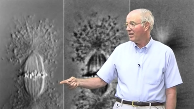
  3. The mitotic spindle produces a good image in polarization microscopy.
    1. Because it is one of the biggest structures in the cell
    2. Because the microtubules are oriented in the same direction and there is a refractive index difference for light traveling parallel versus perpendicular to the spindle axis.
    3. Tubulin has a large refractive index value
    4. The spindle shifts the wavelength of the illuminating light slightly towards the red.
  4. If the mitotic spindle is rotated through 360 degree, how many times will it peak in brightness?
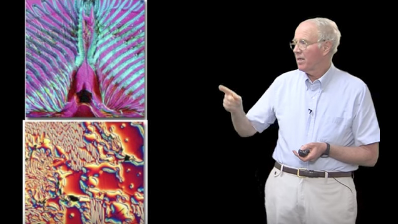
  5. Which of the following is true of using a red plate to measure compensation of a muscle fiber:
    1. The illumination source must be a single wavelength of green light.
    2. If the slow axis of the muscle is aligned with the slow axis of the red plate, then the muscle will appear blue.
    3. The red plate can be used to determine the fast and slow axis of a muscle fiber.
    4. If the slow axis of the muscle is aligned with the slow axis of the red plate, then the muscle will appear yellow.

Answers

View Answers
  1. False.  (The molecular oscillators in the tungsten filament are randomly oriented and hence emit light at all angles.)
  2. B
  3. B
  4. Four
  5. C

Speaker Bio

Ted Salmon

Ted Salmon

Ted Salmon is a Distinguished Professor in the Biology Department at the University of North Carolina. His lab has pioneered techniques in video and digital imaging to study the assembly of spindle microtubules and the segregation of chromosomes during mitosis. Continue Reading

Playlist: Microscopy Series

  • Shinya Inoue Polarized Light and its Interaction with Material
    Polarized Light and its Interaction with Material
  • Differential Interference Contrast (DIC) Microscopy Edward Salmon
    Differential Interference Contrast (DIC) Microscopy
  • Examples of Using Polarization Microscopy: Shinya Inoue
    Examples of Using Polarization Microscopy
  • Microscopy Edward Salmon
    Pragmatics of DIC and Video-Enhanced Contrast Microscopy

Reader Interactions

Leave a Reply Cancel reply

Your email address will not be published. Required fields are marked *

Primary Sidebar

Sign up for the Science Communication Lab education newsletter

  • Sign up Newsletter
  • This field is for validation purposes and should be left unchanged.

Privacy Policy

Help us keep bringing the world’s best biology to you!

Footer

Funders

NSF
NIGMS
Lasker
Rita Allen

Start Here

  • Talks for Everyone
  • Talks for Students
  • Talks for Research
  • Talks for Educators

Explore

  • Explore
  • All Playlists
  • All Speakers
  • All Talks

Talks By Topic

  • Biochemistry
  • Bioengineering
  • Biophysics
  • Cell Biology
  • Development and Stem Cells
  • Ecology
  • Genetics and Gene Regulation
  • Human Disease
  • Immunology
  • Microbiology
  • Neuroscience
  • Plant Biology
  • Techniques

Talks by Series

  • Bench to Bedside
  • Famous Discoveries
  • Great Questions
  • Share Your Research Series

Career

  • Professional Development
  • Career Exploration
  • NRMN Resources
  • Biomedical Workforce

Courses

  • Microscopy Series
  • Short Microscopy Series
  • Open edX Courses
  • Cell Biology Flipped Course
  • Engineering Life Flipped Course
  • Evolution Flipped Course

Educator

  • Educator Registration
  • Educator Resources
  • Log In

About Us

  • About Us
  • iBiology Team
  • Wonder Collaborative
  • Contact Us
  • Mission
  • Privacy Policy
  • SCL Financial Conflict of Interest Policy

This material is based upon work supported by the National Science Foundation and the National Institute of General Medical Sciences under Grant No. 2122350 and 1 R25 GM139147. Any opinion, finding, conclusion, or recommendation expressed in these videos are solely those of the speakers and do not necessarily represent the views of the Science Communication Lab/iBiology, the National Science Foundation, the National Institutes of Health, or other Science Communication Lab funders.

© 2023 - 2006 iBiology · All content under CC BY-NC-ND 3.0 license · Privacy Policy · Terms of Use · Usage Policy
 

Power by iBiology